Describing Data 👨‍💻

MATH 4720/MSSC 5720 Introduction to Statistics

Dr. Cheng-Han Yu
Department of Mathematical and Statistical Sciences
Marquette University

Descriptive Statistics

Data Summary in Tables, Graphics and Numerical Values

Descriptive Statistics (Data Summary)

• Before doing inferential statistics, let’s first learn to understand our data by describing or summarizing it using a table, graph, or some important measures, so that appropriate methods can be performed for better inference results.

Frequency Table for Categorical Variable

• A frequency table (frequency distribution) lists variable values individually for categorical data along with their corresponding number of times occurred in the data (frequencies or counts).

• Frequency table for categorical data with \(n\) data values:

Category name	Frequency	Relative Frequency
\(C_1\)	\(f_1\)	\(f_1/n\)
\(C_2\)	\(f_2\)	\(f_2/n\)
…	…	…
\(C_k\)	\(f_k\)	\(f_k/n\)

Frequency Table for Categorical Variable

• A frequency table (frequency distribution) lists variable values individually for categorical data along with their corresponding number of times occurred in the data (frequencies or counts).

• Example: A categorical variable color that has three categories

Category name	Frequency	Relative Frequency
Red 🔴	8	8/50 = 0.16
Blue 🔵	26	26/50 = 0.52
Black ⚫	16	16/50 = 0.32

R Packages 📦

• Packages wrap up reusable R functions, the documentation that describes how to use them, and data sets all together.

• As of August 2025, there are about 22510 R packages available on CRAN (the Comprehensive R Archive Network)!

• palmerpenguins package

Categorical Frequency Table palmerpenguins package

library(palmerpenguins)

str(penguins)

tibble [344 × 8] (S3: tbl_df/tbl/data.frame)
 $ species          : Factor w/ 3 levels "Adelie","Chinstrap",..: 1 1 1 1 1 1 1 1 1 1 ...
 $ island           : Factor w/ 3 levels "Biscoe","Dream",..: 3 3 3 3 3 3 3 3 3 3 ...
 $ bill_length_mm   : num [1:344] 39.1 39.5 40.3 NA 36.7 39.3 38.9 39.2 34.1 42 ...
 $ bill_depth_mm    : num [1:344] 18.7 17.4 18 NA 19.3 20.6 17.8 19.6 18.1 20.2 ...
 $ flipper_length_mm: int [1:344] 181 186 195 NA 193 190 181 195 193 190 ...
 $ body_mass_g      : int [1:344] 3750 3800 3250 NA 3450 3650 3625 4675 3475 4250 ...
 $ sex              : Factor w/ 2 levels "female","male": 2 1 1 NA 1 2 1 2 NA NA ...
 $ year             : int [1:344] 2007 2007 2007 2007 2007 2007 2007 2007 2007 2007 ...

x <- penguins[, "species"]

Categorical Frequency Table: species

## frequency table
table(x)

species
   Adelie Chinstrap    Gentoo 
      152        68       124 

If we want to create a frequency table shown in definition, which R data structure we can use?

Visualizing a Frequency Table: Bar Chart

barplot(height = table(x), main = "Bar Chart", xlab = "Penguin Species")

Pie Chart

pie(x = table(x), main = "Pie Chart")

Frequency Distribution for Numerical Variables

• Divide the data into \(k\) non-overlapping groups of intervals (classes).

• Convert the data into \(k\) categories with an associated class interval.

• Count the number of measurements falling in a given class interval (class frequency).

Class	Class Interval	Frequency	Relative Frequency
\(1\)	\([a_1, a_2]\)	\(f_1\)	\(f_1/n\)
\(2\)	\((a_2, a_3]\)	\(f_2\)	\(f_2/n\)
…	…	…	…
\(k\)	\((a_k, a_{k+1}]\)	\(f_k\)	\(f_k/n\)

• \((a_2 - a_1) = (a_3 - a_2) = \cdots = (a_{k+1} - a_k)\). All class widths are the same!

Frequency Distribution for Numerical Variables

• Divide the data into \(k\) non-overlapping groups of intervals (classes).

• Convert the data into \(k\) categories with an associated class interval.

• Count the number of measurements falling in a given class interval (class frequency).

Class	Class Interval	Frequency	Relative Frequency
\(1\)	\([80, 100]\)	\(2\)	\(2/50\)
\(2\)	\((100, 120]\)	\(4\)	\(4/50\)
…	…	…	…
\(8\)	\((220, 240]\)	\(3\)	\(3/50\)

Can our grade conversion be used for creating a frequency distribution?

Grade	Percentage
A	[94, 100]
A-	[90, 94)
B+	[87, 90)
B	[83, 87)
B-	[80, 83)
C+	[77, 80)
C	[73, 77)
C-	[70, 73)
D+	[65, 70)
D	[60, 65)
F	[0, 60)

Body Mass (Grams) in Data penguins

body_mass <- penguins$body_mass_g
head(body_mass, 20)

 [1] 3750 3800 3250   NA 3450 3650 3625 4675 3475 4250 3300 3700 3200 3800 4400
[16] 3700 3450 4500 3325 4200

body_mass <- body_mass[complete.cases(body_mass)]

Frequency Distribution of Body Mass

 Class   Class_Intvl Freq Rel_Freq
     1 2700g - 3000g   11     0.03
     2 3000g - 3300g   29     0.08
     3 3300g - 3600g   57     0.17
     4 3600g - 3900g   57     0.17
     5 3900g - 4200g   39     0.11
     6 4200g - 4500g   34     0.10
     7 4500g - 4800g   34     0.10
     8 4800g - 5100g   26     0.08
     9 5100g - 5400g   21     0.06
    10 5400g - 5700g   22     0.06
    11 5700g - 6000g   10     0.03
    12 6000g - 6300g    2     0.01

range(body_mass)

[1] 2700 6300

• All class widths are the same!
• Number of classes should not be too big or too small.
• The lower limit of the 1st class should not be greater than the minimum value of the data.
• The upper limit of the last class should not be smaller than the maximum value of the data.

Wonder how we choose the number of classes or the class width?

R decide the number for us when we visualize the frequency distribution by a histogram.

Visualizing Frequency Distribution by a Histogram

Use default breaks (no need to specify)

hist(x = body_mass, 
     xlab = "Body Mass (gram)",
     main = "Histogram (Defualt)")

Use customized breaks

class_boundary

 [1] 2700 3000 3300 3600 3900 4200 4500 4800 5100 5400 5700 6000 6300

hist(x = body_mass, 
     breaks = class_boundary, #<<
     xlab = "Body Mass (gram)",
     main = "Histogram (Ours)")

Skewness

• Key characteristics of distributions includes shape, center and spread.

• Skewness provides a way to summarize the shape of a distribution.

Remembering Skewness

Is the body mass histogram left skewed or right skewed?

Biostatistics for the Biological and Health Sciences p.53

Scatterplot for Two Numerical Variables

• A scatterplot provides a case-by-case view of data for two numerical variables.

plot(x = penguins$bill_length_mm, y = penguins$bill_depth_mm,
     xlab = "Bill Length", ylab = "Bill Depth",
     pch = 16, col = 4)

For the penguins data, do

• Pie chart for variable island.
• Histogram for variable flipper_length_mm. Discuss its shape.
• Scatter plot for variables flipper_length_mm and bill_length_mm.

02:00

Numerical Summaries of Data

If you need to choose one value that represents the entire data, what value would you choose?

• Measure of Center: We typically use the middle point. (What does “middle” mean?)

• Measure of Variation: What values tell us how much variation a variable has?

Measures of Center: Mean

• The (arithmetic) mean or average is adding up all of the values, then dividing by the total number of them.

• Let \(x_1, x_2, \dots, x_n\) denote the measurements observed in a sample of size \(n\). Then the sample mean is defined as \[\overline{x} = \frac{\sum_{i=1}^{n} x_i}{n} = \frac{x_1 + x_2 + \dots + x_n}{n}\]

• In the body mass example, \[\overline{x} = \frac{3750 + 3800 + \cdots + 3775}{342} = 4202\]

mean(body_mass)

[1] 4202

• Mean balances data Values. It means that the sum of deviations from the mean is 0.

Balancing Point

• Think of the mean as the balancing point of the distribution.

• Mean is a measure of center in the sense that it can be viewed as the balancing point of the distribution.
• This is the distribution of the interest rate.
• And if you imagine that we put all those data points on a see-saw, the sample mean is the balancing point that keeps the see-saw balanced horizontally.

Measures of Center: Median

• Median: the middle value when data values are sorted.

• Half of the values are less than or equal to the median, and the other half are greater than it.

• To find the median, we first sort the values.

• \(n\) is odd: the median is located in the exact middle of the ordered values.

  • Data: (0, 2, 10, 14, 8)
  • Sorted Data: (0, 2, 8, 10, 14)
  • The median is \(8\)

• \(n\) is even: the median is the average of the two middle numbers.
  • Data: (0, 2, 10, 14, 8, 12)
  • Sorted Data: (0, 2, 8, 10, 12, 14)
  • The median is \(\frac{8 + 10}{2} = 9\)

• The Median is the middle value when data values are sorted from the lowest to highest.

• Half of the values are less than or equal to the median, and the other half are greater than it.

• To find the median (well without using any technology or computer), we first sort the values.

• If \(n\) is odd, the median is located in the exact middle of the ordered values.

• There are two on its right and two on its left. it is right on the middle.

• If \(n\) is even, the median is the average of the two middle numbers.

• 8 or 10 itself is not right on the middle.

Calculate Median in R

median(body_mass)  ## Compute the median using command median()

[1] 4050

(sort_mass <- sort(body_mass))  ## sort data

  [1] 2700 2850 2850 2900 2900 2900 2900 2925 2975 3000 3000 3050 3050 3050 3050
 [16] 3075 3100 3150 3150 3150 3150 3175 3175 3200 3200 3200 3200 3200 3250 3250
 [31] 3250 3250 3250 3275 3300 3300 3300 3300 3300 3300 3325 3325 3325 3325 3325
 [46] 3350 3350 3350 3350 3350 3400 3400 3400 3400 3400 3400 3400 3400 3425 3425
 [61] 3450 3450 3450 3450 3450 3450 3450 3450 3475 3475 3475 3500 3500 3500 3500
 [76] 3500 3500 3500 3525 3525 3550 3550 3550 3550 3550 3550 3550 3550 3550 3575
 [91] 3600 3600 3600 3600 3600 3600 3600 3625 3650 3650 3650 3650 3650 3650 3675
[106] 3675 3700 3700 3700 3700 3700 3700 3700 3700 3700 3700 3700 3725 3725 3725
[121] 3750 3750 3750 3750 3750 3775 3775 3775 3775 3800 3800 3800 3800 3800 3800
[136] 3800 3800 3800 3800 3800 3800 3825 3850 3875 3900 3900 3900 3900 3900 3900
[151] 3900 3900 3900 3900 3950 3950 3950 3950 3950 3950 3950 3950 3950 3950 3975
[166] 4000 4000 4000 4000 4000 4050 4050 4050 4050 4050 4050 4075 4100 4100 4100
[181] 4100 4100 4150 4150 4150 4150 4150 4150 4200 4200 4200 4200 4200 4250 4250
[196] 4250 4250 4250 4275 4300 4300 4300 4300 4300 4300 4300 4300 4350 4350 4375
[211] 4400 4400 4400 4400 4400 4400 4400 4400 4450 4450 4450 4450 4450 4475 4500
[226] 4500 4500 4550 4550 4575 4600 4600 4600 4600 4600 4625 4625 4650 4650 4650
[241] 4650 4650 4675 4700 4700 4700 4700 4700 4700 4725 4725 4725 4750 4750 4750
[256] 4750 4750 4775 4800 4800 4800 4850 4850 4850 4850 4875 4875 4875 4900 4900
[271] 4925 4925 4950 4950 4975 5000 5000 5000 5000 5000 5000 5050 5050 5050 5100
[286] 5100 5100 5150 5150 5200 5200 5200 5200 5250 5250 5250 5300 5300 5300 5300
[301] 5350 5350 5350 5400 5400 5400 5400 5400 5450 5500 5500 5500 5500 5500 5550
[316] 5550 5550 5550 5550 5550 5600 5600 5650 5650 5650 5700 5700 5700 5700 5700
[331] 5750 5800 5800 5850 5850 5850 5950 5950 6000 6000 6050 6300

length(body_mass)  ## Check sample size is odd or even

[1] 342

(sort_mass[171] + sort_mass[172]) / 2  ## Verify the answer

[1] 4050

(body_mass[171] + body_mass[172]) / 2  ## Using un-sorted data leads to a wrong answer!!

[1] 5525

Measures of Center: Mode

• Mode: the value that occurs most frequently.

• For continuous numerical data, it is common to have no observations with the same value.

• Practical definition: A mode is represented by a prominent peak in the distribution.

## Create a frequency table 
table_data <- table(body_mass)

## Sort the table to find the mode that occurs most frequently
## the number that happens most frequently will be the first one
sort(table_data, decreasing = TRUE)

body_mass
3800 3700 3900 3950 3550 3400 3450 4300 4400 3500 3600 3300 3650 4050 4150 4700 
  12   11   10   10    9    8    8    8    8    7    7    6    6    6    6    6 
5000 5550 3200 3250 3325 3350 3750 4000 4100 4200 4250 4450 4600 4650 4750 5400 
   6    6    5    5    5    5    5    5    5    5    5    5    5    5    5    5 
5500 5700 2900 3050 3150 3775 4850 5200 5300 3475 3725 4500 4725 4800 4875 5050 
   5    5    4    4    4    4    4    4    4    3    3    3    3    3    3    3 
5100 5250 5350 5650 5850 2850 3000 3175 3425 3525 3675 4350 4550 4625 4900 4925 
   3    3    3    3    3    2    2    2    2    2    2    2    2    2    2    2 
4950 5150 5600 5800 5950 6000 2700 2925 2975 3075 3100 3275 3575 3625 3825 3850 
   2    2    2    2    2    2    1    1    1    1    1    1    1    1    1    1 
3875 3975 4075 4275 4375 4475 4575 4675 4775 4975 5450 5750 6050 6300 
   1    1    1    1    1    1    1    1    1    1    1    1    1    1 

• Mathematically, the mode is the value in the data that occurs most frequently.
• For continous numerical data that take on infinitely many possible values, it is common to have no observations with the same value in a data set, making this definition impractical.
• Practical definition: A mode is represented by a prominent peak in the distribution.

Comparison of Mean, Median and Mode

• Mean is sensitive to extreme values (outliers).

• Median/mode is more robust than mean.

head(data_extreme, 10)

 [1] 37500  3800  3250  3450  3650  3625  4675  3475  4250  3300

mean(data_extreme)  ## Large mean! Original mean is 4202

[1] 4300

median(data_extreme)  ## Median does not change!

[1] 4050

names(sort(table(data_extreme), decreasing = TRUE))[1] ## Mode does not change too!

[1] "3800"

• Mean is sensitive to extreme values (outliers).
• Median/mode is more robust than mean, meaning that median and mode will not change or not change much if few data values change.

Comparison of Mean, Median and Mode

• Mode is applicable for both categorical and numerical data, while median and mean work for numerical data only.

• There may be more than one mode, but there is only one median and one mean.

• Mode is applicable for both categorical and numerical data, while median and mean work for numerical data only.
  • Show Categorical homeownership freq table
  • Show int_rate mode
• There may be more than one mode, but there is only one median and one mean.
• mean is sensitive to extreme values. The values at the long tails are extreme values comparing to the values in the middle.
• This forces the mean to be pulled toward the left in order to balance the data.
• Mode happens at the peak of the distribution

Measures of Variation

• Done the discussion of measure of center.
• Now let’s see how we quantify the variation of data.
• Here we have three frequency distributions with the same mean, median and mode because their distribution is symmetric.
• But from top to bottom, the data have small, median and large variation.
• Basically larger variation means the data values spread out more.
• So although the data mean is right here, but in general, data values are not very close to the mean. Their deviation from the sample mean is large. OK.

Measures of Variation: p-th percentile

• p-th percentile (quantile): a data value such that
  • at most \(p\%\) of the values are below it
  • at most \((1-p)\%\) of the values are above it

• Two datasets with the same mean 20.
  • One data set has 99-th percentile = 30, and 1-st percentile = 10.
  • The other has 99-th percentile = 40, and 1-st percentile = 0.
• Which data have larger variation?

https://en.wikipedia.org/wiki/ACT_(test)

• The first Measure of Variation is p-th percentile
• p-th percentile (quantile): a data value such that
  • at most \(p\%\) of the values are below it
  • at most \((1-p)\%\) of the values are above it

Measures of Variation: Interquartile Range (IQR)

• First Quartile (Q1): the 25-th percentile

• Second Quartile (Q2): the 50-th percentile (Median)

• Third Quartile (Q3): the 75-th percentile

• Interquartile Range (IQR): Q3 - Q1

## Use quantile() to find any percentile 
## through specifying the probability
quantile(x = body_mass, 
         probs = c(0.25, 0.5, 0.75))

 25%  50%  75% 
3550 4050 4750 

## IQR by definition
quantile(x = body_mass, probs = 0.75) - 
  quantile(x = body_mass, probs = 0.25) 

 75% 
1200 

## IQR()
IQR(body_mass)  

[1] 1200

## summary() to get the numeric summary
summary(body_mass)

   Min. 1st Qu.  Median    Mean 3rd Qu.    Max. 
   2700    3550    4050    4202    4750    6300 

Larger IQR means more or less variation?

The range of the middle 50% of the data.

Variance and Standard Deviation

• The distance of an observation from its mean, \(x_i - \overline{x}\), its deviation.

• Sample Variance is defined as \[ s^2 = \frac{\sum_{i=1}^n(x_i - \overline{x})^2}{n-1} \]

• Sample Standard Deviation (SD) is defined as the square root of the variance \[ s = \sqrt{\frac{\sum_{i=1}^n(x_i - \overline{x})^2}{n-1}} \]

• Variance is the average of squared deviation from the sample mean \(\overline{x}\) or the mean squared deviation from the mean.

• SD is the root mean squared deviation from the mean. It measures, on average, how far the data spread out around the average.

Compute Variance and SD

var(body_mass)

[1] 643131

sqrt(var(body_mass))

[1] 802

sd(body_mass)

[1] 802

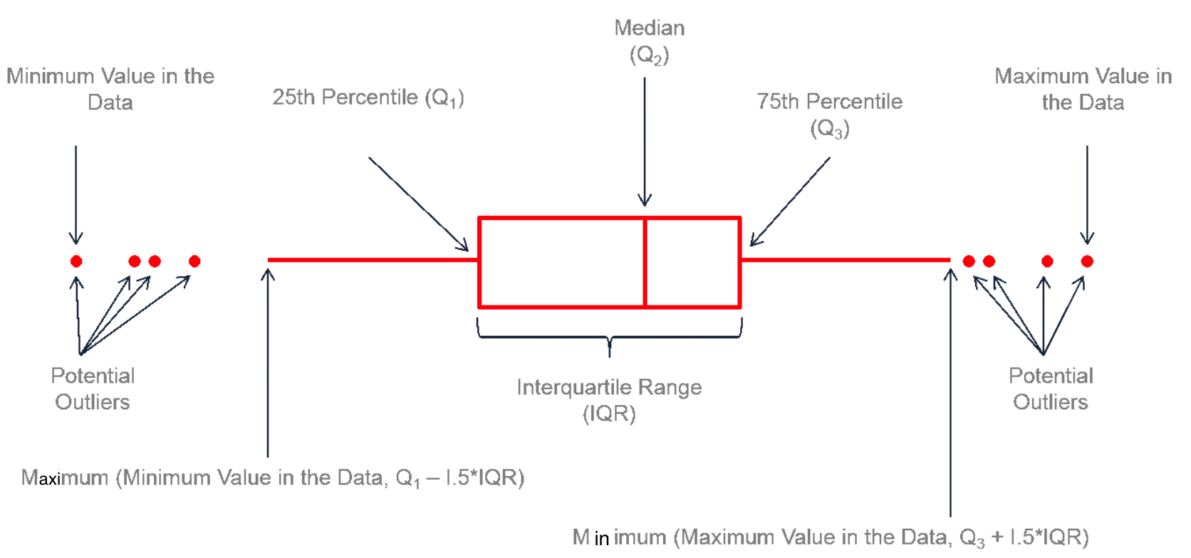
Visualizing Data Variation: Boxplot

When plotting the whiskers,

• minimum value in the data means the minimal value that is not an potential outlier.

• maximum value in the data means the maximal value that is not an potential outlier.

https://www.leansigmacorporation.com/box-plot-with-minitab/

• To Visualize Data Variation, we can make a so-called Boxplot.
• The plot has a box in the middle, and so-called whiskers that are these two straight lines connected to the box.
• Let’s look at the box first. We have 3 vertical lines here. The lines from left to right indicate Q1, Q2 or the median, and Q3.
• So the length of the box shows the IQR.
• Now let’s look at the whiskers.
• The upper limit of the whisker is the smaller one of the maximum of values and Q3 + 1.5 IQR
• The lower limit of the whisker on the left is the larger one of the minimum of values and Q1 - 1.5 IQR
• For any data values that are greater than Q3 + 1.5 IQR or smaller than Q1 - 1.5 IQR, we show them as a point.
• Basically those points are far from the center of the data, and we could potentially treat them as extreme values or outliers.

Body Mass Boxplot

• Here shows the boxplot of the interest rate data.
• You can see that there are two very high interest rates in the data. They are 25% or more.
• And the median interest rate is just about 10%. And so these two data points are suspected outliers. They are way far from the the median or the most data points.
• If

Boxplot in R

boxplot(body_mass, ylab = "Body Mass (g)")

range(body_mass)

[1] 2700 6300

Q3 <- quantile(body_mass, probs = 0.75, 
               names = FALSE)
Q1 <- quantile(body_mass, probs = 0.25, 
               names = FALSE)
IQR <- Q3 - Q1
Q1 - 1.5 * IQR

[1] 1750

Q3 + 1.5 * IQR

[1] 6550

• In R, we can create a boxplot using boxplot(). sort(int_rate, decreasing = TRUE)[1:5] sort(int_rate)[1:5]

For the penguins data,

• Make a boxplot for the variable bill_depth_mm.

• Compute the minimum, Q1, Q2, Q3, and maximum values of bill_depth_mm. (Hint: summary() function is pretty useful! 👍)

02:00