Statistical Inference: Point and Interval Estimation

MATH 4720/MSSC 5720 Introduction to Statistics

Dr. Cheng-Han Yu
Department of Mathematical and Statistical Sciences
Marquette University

Foundations for Inference

• Estimation: Point and Interval Estimation

• Testing

Inference Framework

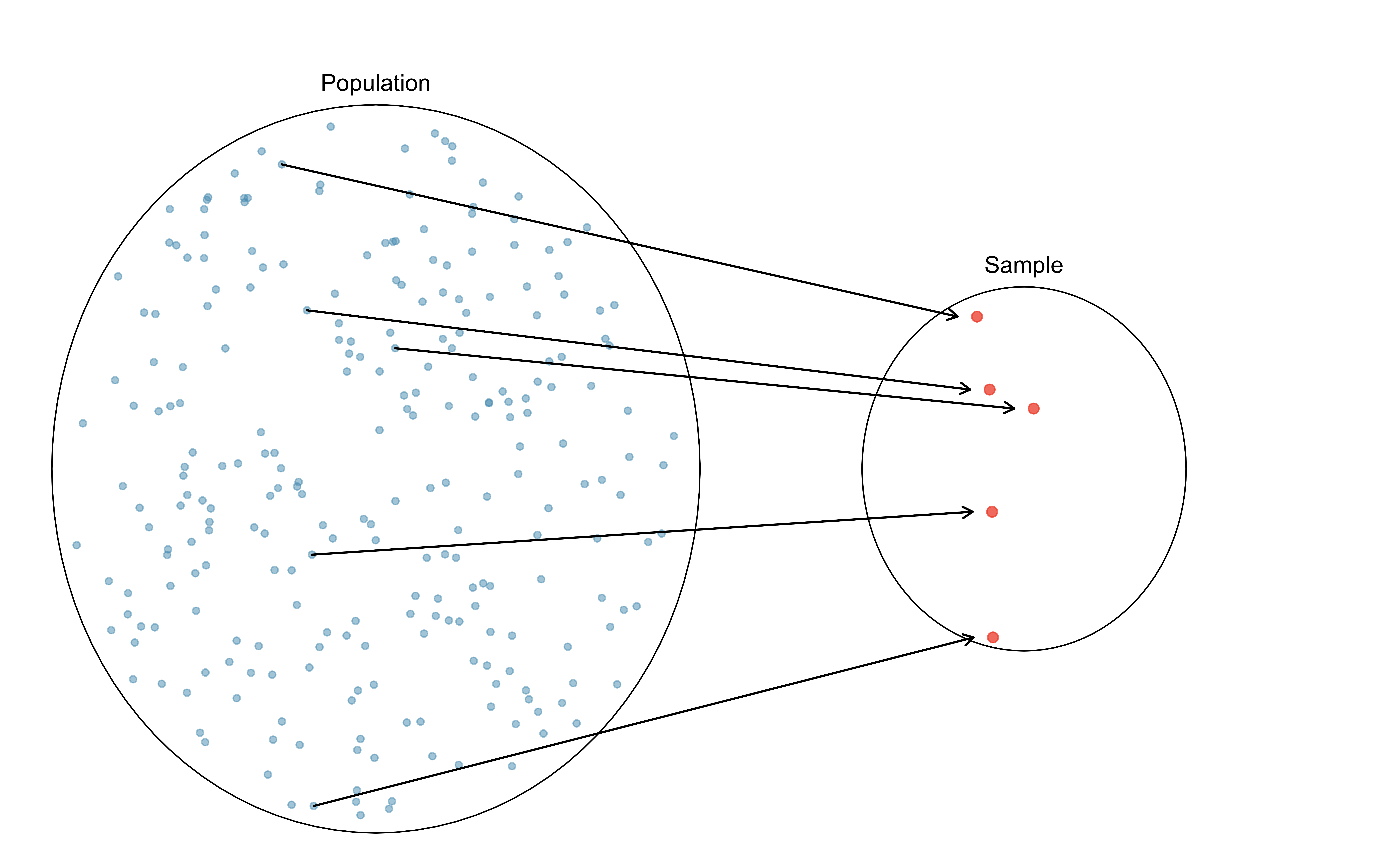
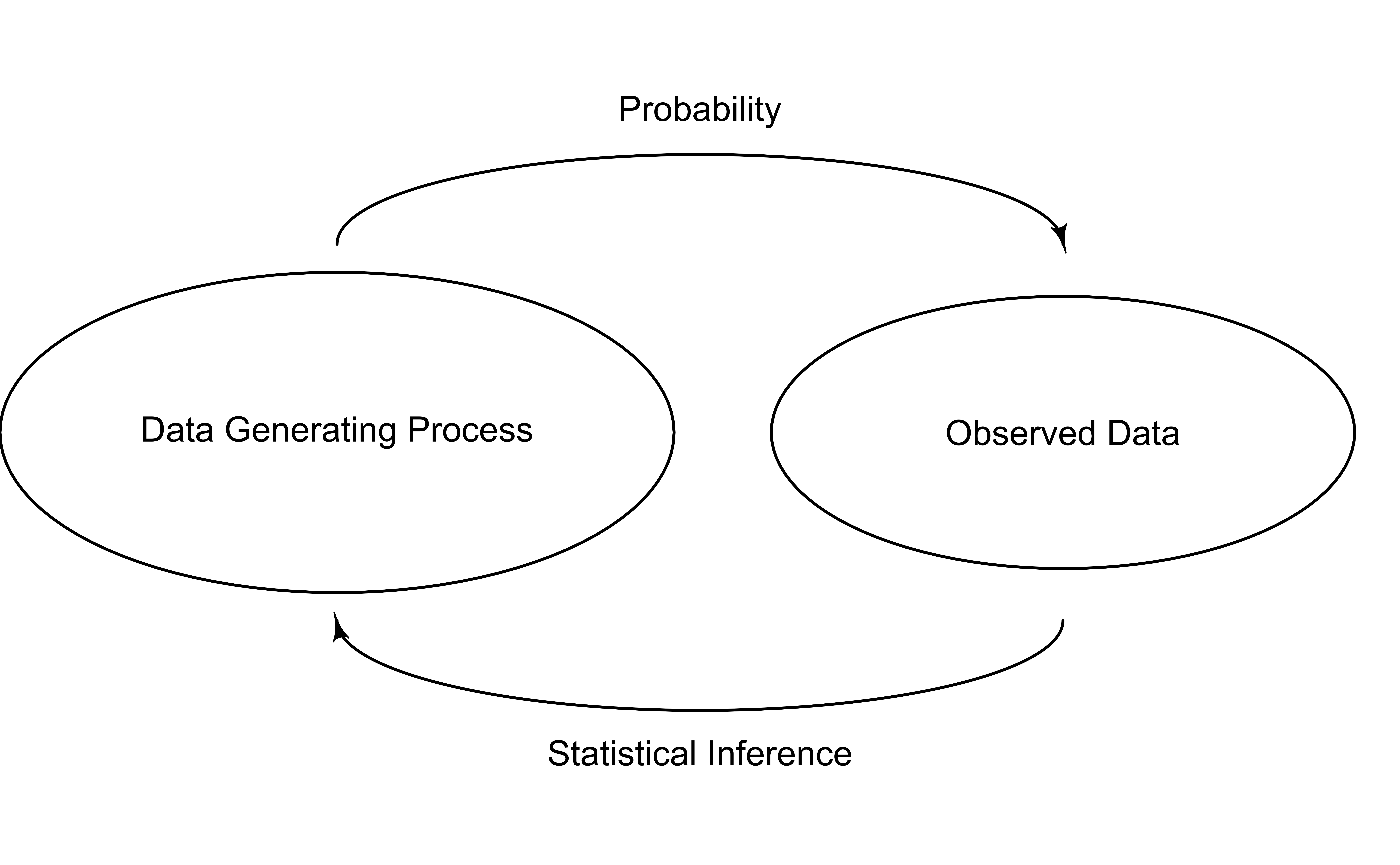
• Inferential statistics uses sample data to learn about an unknown population.

• Idea: Assume the target population follows some distribution but with unknown parameters.

  • Assume the population is normally distributed, but don’t know its mean and/or variance. Marquette students’ mean GPA for example.

• Goal: Learning the unknown parameters of the assumed population distribution.

• Two approaches in parameter learning: Estimation and Hypothesis testing.

• We finally are going to study inferential statistics that uses sample data to learn about an unknown population. (Getting harder! Be careful!)
• We are interested in learning unknown parameters of the assumed population distribution, since knowledge of the parameters yield knowledge of the entire population.
• In parameter learning, we consider two approaches, estimation and hypothesis testing.
  • Learn the mean and/or variance of the normal distribution.

Point Estimator

If you can use only one single number to guess the unknown population mean \(\mu\), what would you like to use?

The one single point used to estimate the unknown parameter is called a point estimator.

• A point estimator is any function of data \((X_1, X_2, \dots, X_n)\) (Before actually being collected).

  • Any statistic is a point estimator.

• A point estimate is a value of a point estimator used to estimate a population parameter. (A value calculated using the collected data).

• Sample mean \((\overline{X})\) is a statistic and a point estimator for the population mean \(\mu\).

• A point estimator is any function of a sample \((X_1, X_2, \dots, X_n)\).
  • Any statistic is a point estimator.
• A point estimate is a value of a point estimator used to estimate a population parameter.
• Sample mean \((\overline{X})\) is a statistic and a point estimator for the population mean \(\mu\).

Sample Mean as an Point Estimator

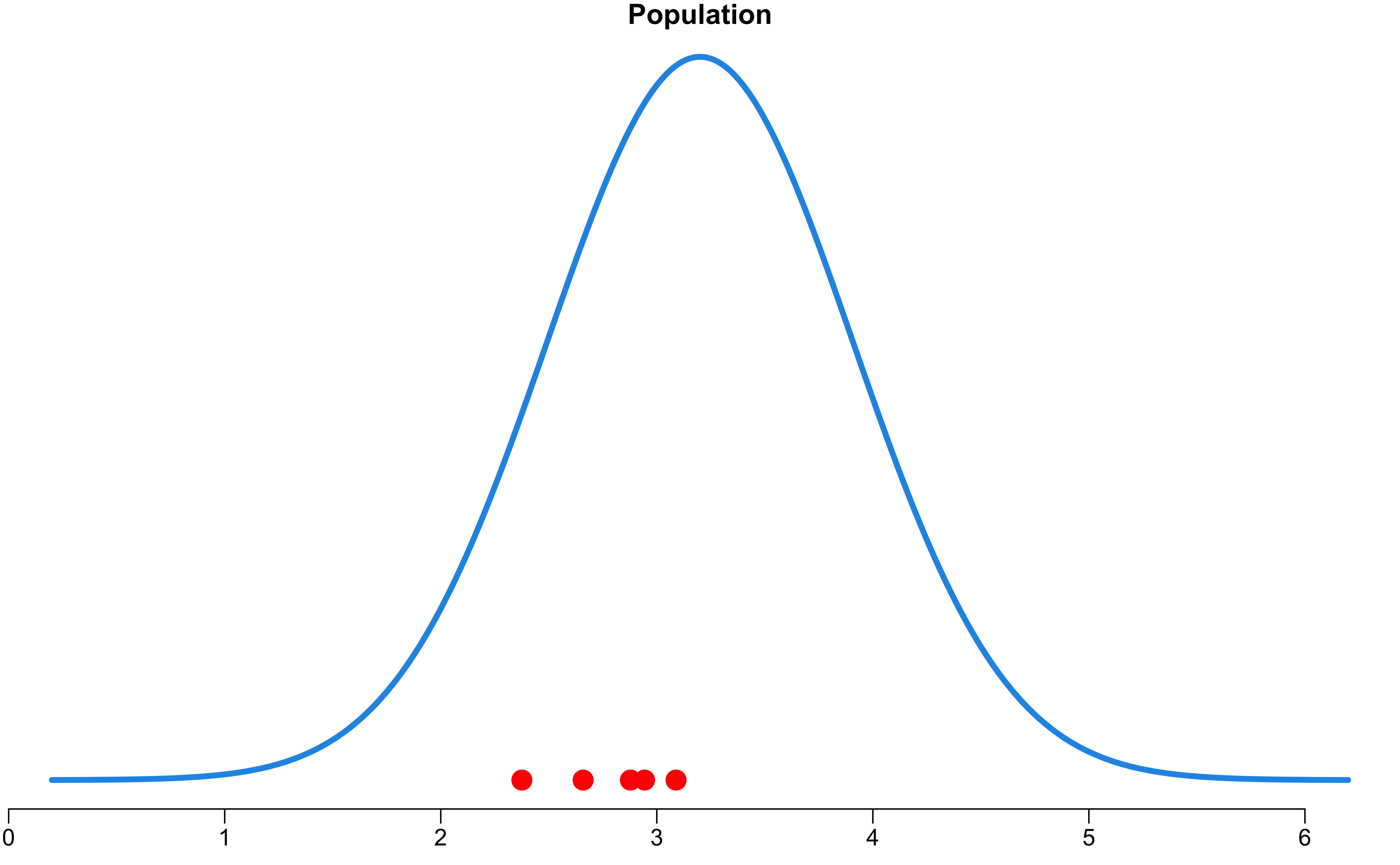
• Draw 5 values from the population that follows \(N(3.2, 0.5)\) as sample data \((x_1, x_2, x_3, x_4, x_5)\).

x1	x2	x3	x4	x5	sample mean
2.88	2.94	3.09	2.66	2.38	2.79

• \(\mu = 3.2\), and we use the point estimate \(\overline{x}=\) 2.79 to estimate it.

Why \(\overline{x}\) is not equal to \(\mu\)?

Due to its randomness nature

• Due to the randomness nature of drawing a sample value from the population distribution, we do not expect the statistic to be the same as the corresponding parameter.

Variability in Estimates

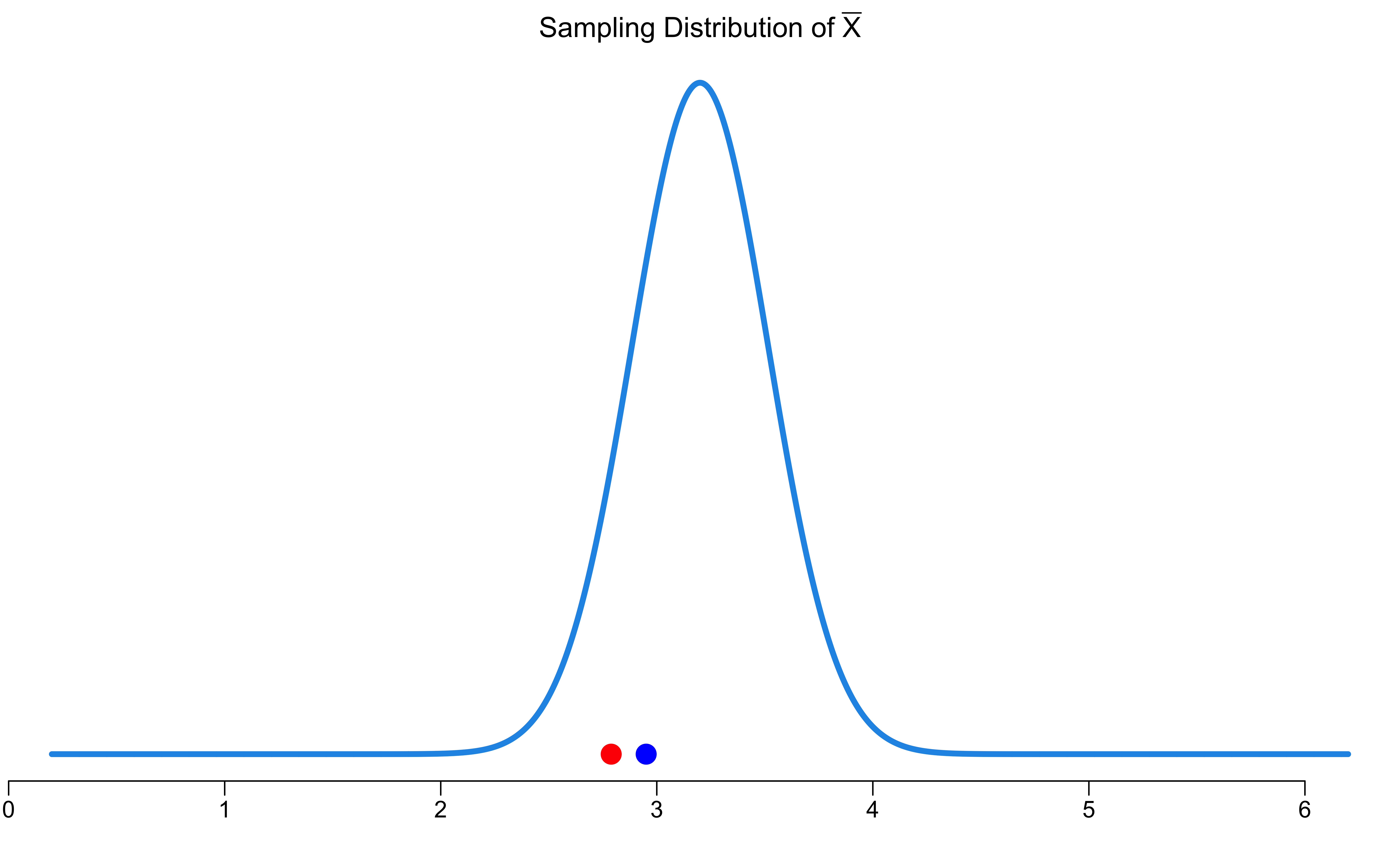
• If another sample of size \(5\) is drawn from the same population:

x1	x2	x3	x4	x5	sample mean
2.35	3.4	3.97	1.54	3.5	2.95

• The second sample mean \(\overline{x} =\) 2.95 is different from the first one.

Why the first sample and the second sample give us different sample means?

A point estimator has its own sampling distribution

• A statistic value (point estimate) calculated from a sample varies from sample to sample because a point estimator is also a random variable, and it has its own sampling distribution! (why we learn sampling distribution. it measures the variation of a point estimator)

Why Point Estimates Are Not Enough

If you want to estimate \(\mu\), do you prefer to report a range of values the parameter might be in, or a single estimate like \(\overline{x}\)?

If you want to catch a fish, do you prefer a spear or a net?

• Due to variation of \(\overline{X}\), if we report a point estimate \(\overline{x}\), we probably won’t hit the exact \(\mu\).
• If we report a range of plausible values, we have a better shot at capturing the parameter!

• the estimate \(\overline{x}\) may not be precise or reliable.

Confidence Intervals

A plausible range of values for \(\mu\) is called a confidence interval (CI).

• To construct a CI we need to quantify the variability of our sample mean.

• Quantifying this uncertainty requires a measurement of how much we would expect the sample statistic to vary from sample to sample.

  • That is the variance of the sampling distribution of the sample mean!

• To construct a CI we need to quantify the variability of our sample mean because the variability determines the upper and lower bound of the range of the plausible values.
• The variability of the sample mean determines the size of CI.
• This range depends on how precise and reliable our \(\overline{X}\) is as an estimate of \(\mu\).
• If the variation of our sample mean is pretty large, meaning that every time we collect a sample, the sample mean varies a lot from one to another, then we are more uncertain about the value of \(\mu\).
• And that mean the plausible range of values for \(\mu\) will be pretty wide, or the CI will be much wider.

👉 The larger variation of \(\overline{X}\) is, the wider the CI for \(\mu\) will be, given the same “level of confidence”.

Do we know the variance of \(\overline{X}\)?

• By CLT, \(\overline{X} \sim N(\mu, \sigma^2/n)\) regardless of what the population distribution is.

Confidence Interval Is for a Parameter

• A confidence interval is for a parameter, NOT a statistic.

  • Use the sample mean to form a confidence interval for the population mean.

• We never say “The confidence interval of the sample mean \(\overline{X}\) is …”

• We say “The confidence interval for the true population mean \(\mu\) is …”

• In general, a confidence interval for \(\mu\) has the form

\(\large \overline{x} \pm m = (\overline{x} - m, \overline{x} + m)\)

• The \(m\) is called margin of error.

• \(\overline{x} - m\) is the lower bound and \(\overline{x} + m\) is the upper bound of the confidence interval.

• The point estimate \(\overline{x}\) and margin of error \(m\) can be obtained from known quantities and our data once sampled.

• Use the sample variance to form a confidence interval for the population variance.

Precision vs. Reliability

If we want to be very certain that we capture \(\mu\), should we use a wider or a narrower interval? What drawbacks are associated with using a wider interval?

• Here is a question. If we want to be very certain that we capture the population parameter, should we use a wider or a narrower interval?
• We use a wider interval because a wider interval is more likely to capture the population parameter value. So a 99% confidence interval is wider than a 95% confidence interval.
• But What drawbacks are associated with using a wider interval?

• Let’s look at this comic.
• I can say I am 100% confident that your exam 1 score is between 0 and 100. Am I right? Yes. But do I provide helpful information? Absolutely not, the interval includes every possible score of the exam. The interval is too wide to be helpful.

With the sample size fixed, precision and reliability have a trade-off relationship.

.question[ How can we get best of both worlds – high precision and high reliability/accuracy?] - How can we get best of both worlds – high precision and high reliability/accuracy, meaning short interval with high level of confidence. - What we need is larger sample size, given that the sample quality is good. - Easy statement, but sometimes it’s hard to collect more samples.

\((1 - \alpha)100\%\) Confidence Intervals

• The confidence level \(1-\alpha\): the proportion of times that the CI contains the population parameter, assuming that the estimation process is repeated a large number of times.

• The common choices for the confidence level are

  • 90% \((\alpha = 0.10)\)
  • 95% \((\alpha = 0.05)\)
  • 99% \((\alpha = 0.01)\)

• 95% is the most common level because of good balance between precision (width of the CI) and reliability (confidence level)

• High reliability and Low precision. I am 100% confident that the mean height of Marquette students is between 3’0” and 8’0”. duh…🤷

• Low reliability and High precision. I am 20% confident that mean height of Marquette students is between 5’6” and 5’7”. far from it…🙅

• A confidence interval is associated with a confidence level.
• The confidence level (often expressed as the percentage value, such as 95%)

\(95\%\) Confidence Intervals for \(\mu\): Z-score

• \(\alpha = 0.05\)

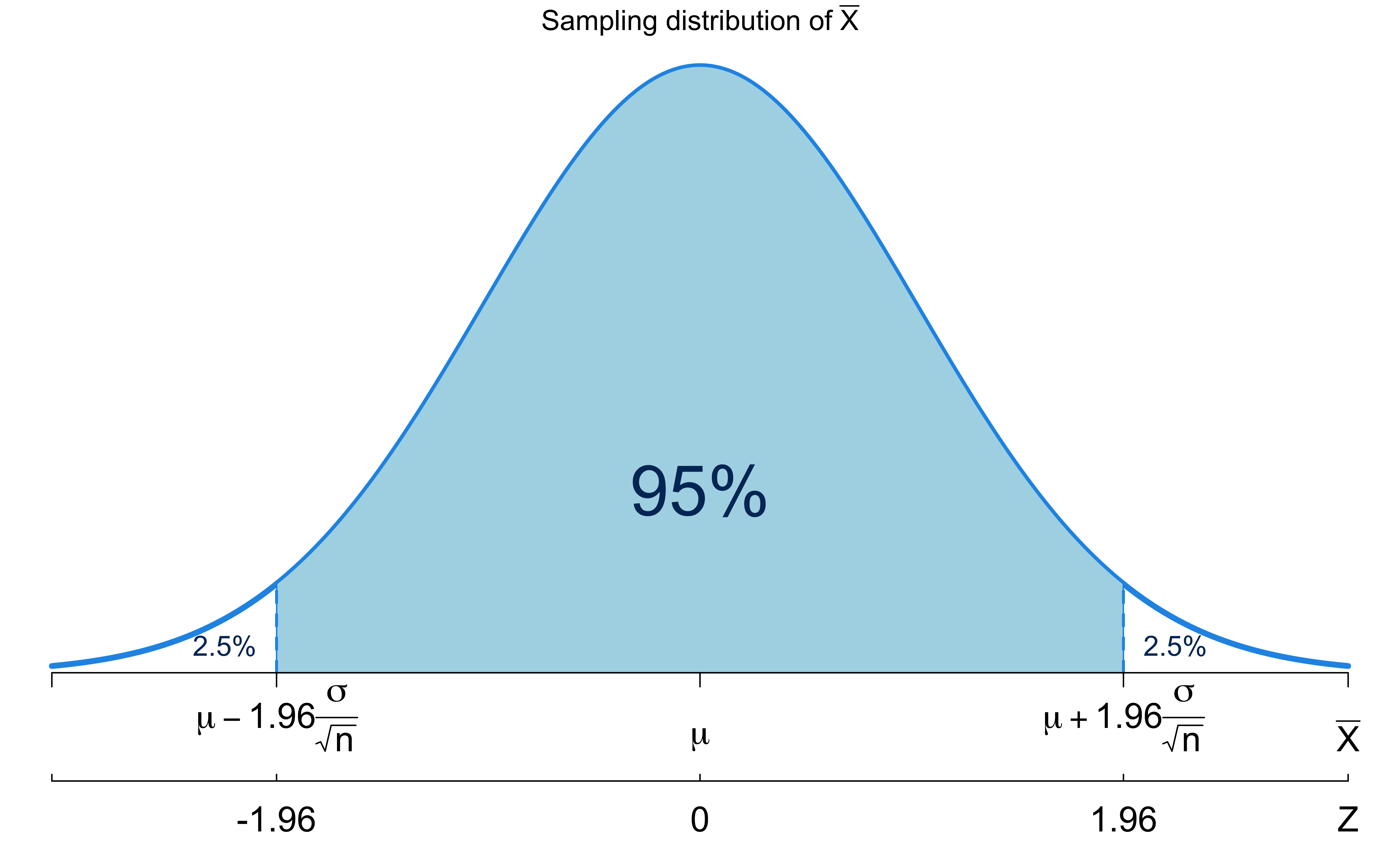
• Start with the sampling distribution of \(\overline{X} \sim N\left(\mu, \frac{\sigma^2}{n}\right)\)

• \(\overline{x}\) will be within 1.96 SDs of the population mean \(\mu\) \(95\%\) of the time.

• The \(z\)-score of 1.96 is associated with 2.5% area to the right, and called a critical value denoted as \(z_{0.025}\).

(and Z = -1.96 has 2.5% area to the left); -At a distance of zα/2 standard deviations to the right of μ, there is an area of α/2 under the normal density curve.

\(95\%\) Confidence Intervals for \(\mu\): Probability

\[P\left(\mu-1.96\frac{\sigma}{\sqrt{n}} < \overline{X} < \mu + 1.96\frac{\sigma}{\sqrt{n}} \right) = 0.95\]

Is the interval \(\left(\mu-1.96\frac{\sigma}{\sqrt{n}}, \mu+1.96\frac{\sigma}{\sqrt{n}} \right)\) our confidence interval?

❌ No! We don’t know \(\mu\), the quantity we like to estimate!

But we’re almost there!

\(95\%\) Confidence Intervals for \(\mu\): Formula

\[ \small P\left(\mu-1.96\frac{\sigma}{\sqrt{n}} < \overline{X} < \mu + 1.96\frac{\sigma}{\sqrt{n}} \right) = 0.95 \iff P\left( \boxed{\overline{X}-1.96\frac{\sigma}{\sqrt{n}} < \mu < \overline{X} + 1.96\frac{\sigma}{\sqrt{n}}} \right) = 0.95\]

• With sample data of size \(n\), \(\left(\overline{x}-1.96\frac{\sigma}{\sqrt{n}}, \overline{x} + 1.96\frac{\sigma}{\sqrt{n}}\right)\) is our \(95\%\) CI for \(\mu\) if \(\sigma\) is known to us!

• The margin of error \(m = 1.96\frac{\sigma}{\sqrt{n}}\).

Confidence Intervals for population Means: Known Variance Case

Confidence Intervals for \(\mu\) When \(\sigma\) is Known

Requirements for estimating \(\mu\) when \(\sigma\) is known:

• 👉 The sample should be a random sample, i.e. All data \(X_i\) are drawn from the same population, and \(X_i\) and \(X_j\) are independent.

  • Any methods in the course are based on a random sample

• 👉 The population standard deviation \(\sigma\) is known.

• 👉 The population is either normally distributed or \(n > 30\) or both, i.e., \(X_i \sim N(\mu, \sigma^2)\).

  • \(n > 30\) allows CLT to be applied and hence normality is satisfied.

\((1-\alpha)100\%\) Confidence Intervals for \(\mu\):

\(\left(\overline{x}-1.96\frac{\sigma}{\sqrt{n}}, \overline{x} + 1.96\frac{\sigma}{\sqrt{n}}\right)\) \(\left(\overline{x}-z_{0.025}\frac{\sigma}{\sqrt{n}}, \overline{x} + z_{0.025}\frac{\sigma}{\sqrt{n}}\right)\)

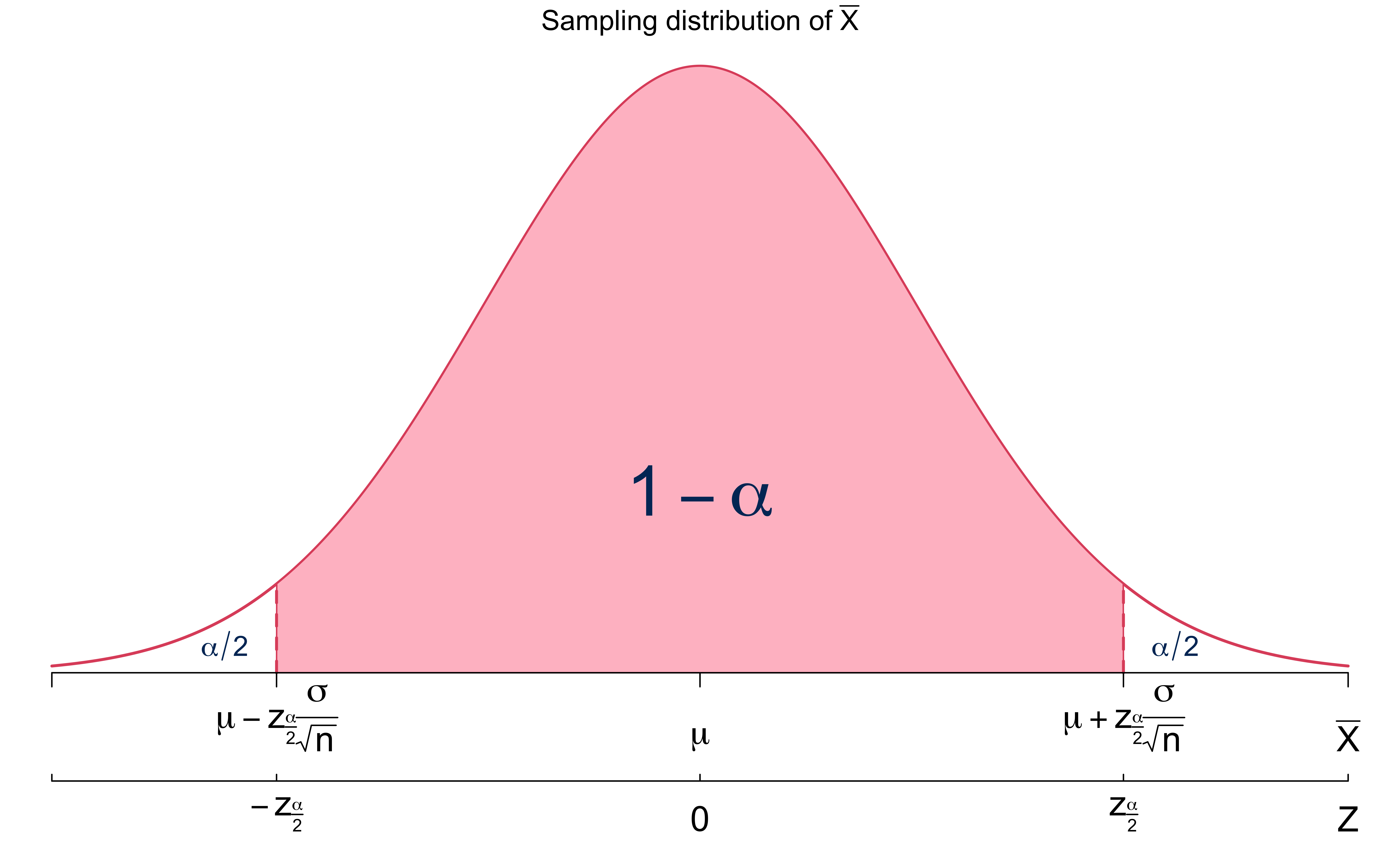
\(\left(\overline{x}-z_{\alpha/2}\frac{\sigma}{\sqrt{n}}, \overline{x} + z_{\alpha/2}\frac{\sigma}{\sqrt{n}}\right)\)

Confidence Intervals for \(\mu\) When \(\sigma\) is Known

Procedures for constructing a confidence interval for \(\mu\) when \(\sigma\) known:

1. Check that the requirements are satisfied.
   
   
2. Decide \(\alpha\) or confidence level \((1 - \alpha)\).
   
   
3. Find the critical value \(z_{\alpha/2}\).
   
   
4. Evaluate margin of error \(m = z_{\alpha/2} \cdot \frac{\sigma}{\sqrt{n}}\)
   
   
5. Construct the \((1 - \alpha)100\%\) CI for \(\mu\) using sample mean \(\overline{x}\) and margin of error \(m\):

\[\left( \overline{x} -z_{\alpha/2}\frac{\sigma}{\sqrt{n}}, \, \overline{x} + z_{\alpha/2} \frac{\sigma}{\sqrt{n}}\right)\]

Example: CI for \(\mu\) When \(\sigma\) is Known

We want to know the mean systolic blood pressure (SBP) of a population.

• Assume that the population distribution is normal with the standard deviation of 5 mmHg.

• We have a random sample of 16 subjects of this population with mean 121.5.

• Estimate the mean SBP with a 95% confidence interval.

1. Requirements: Normality is assumed, \(\sigma = 5\) is known and a random sample is collected.

2. Decide \(\alpha\): \(\alpha = 0.05\)

3. Find the critical value \(z_{\alpha/2}\): \(z_{\alpha/2} = z_{0.025} = 1.96\)

4. Evaluate margin of error \(m = z_{\alpha/2} \frac{\sigma}{\sqrt{n}}\): \(m = (1.96) \frac{5}{\sqrt{16}} = 2.45\)

5. Construct the \((1 - \alpha)100\%\) CI: The 95% CI for the mean SBP is \(\overline{x} \pm z_{\alpha/2}\frac{\sigma}{\sqrt{n}} = (121.5 -2.45, 121.5 + 2.45) = (119.05, 123.95)\)

Computation in R

## save all information we have
alpha <- 0.05
n <- 16
x_bar <- 121.5
sig <- 5

## 95% CI
## z-critical value
(cri_z <- qnorm(p = alpha / 2, lower.tail = FALSE))  

[1] 1.96

## margin of error
(m_z <- cri_z * (sig / sqrt(n)))  

[1] 2.45

## 95% CI for mu when sigma is known
x_bar + c(-1, 1) * m_z  

[1] 119.1 123.9

Construct a 99% CI for the mean SBP. Do you expect to have a wider or narrower interval? Why?

Interpreting a Confidence Interval

• “We are 95% confident that the mean SBP lies between 119.1 mm and 123.9 mm.”

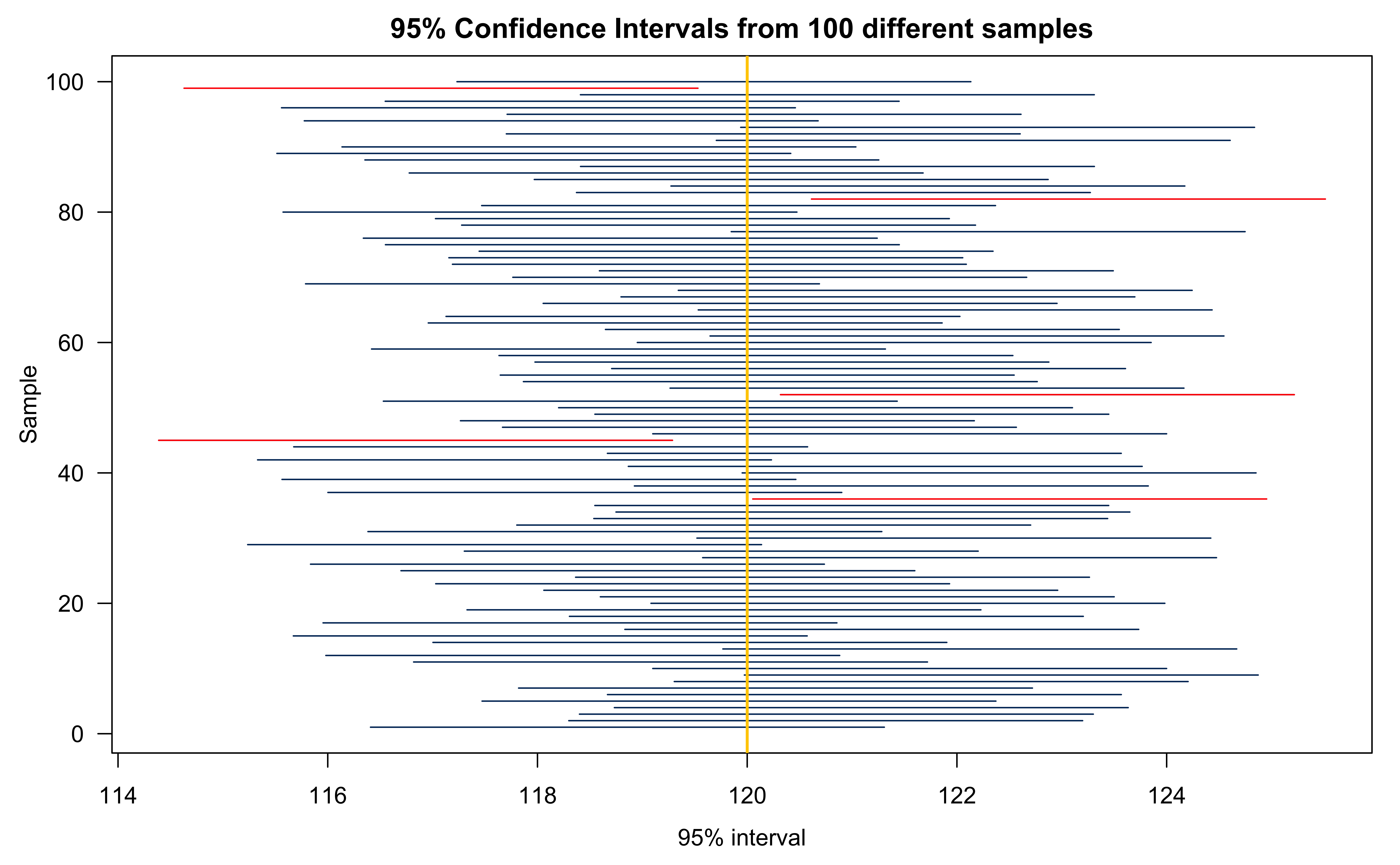
• Suppose we were able to collect our dataset many times and build the corresponding CIs.

• We would expect about 95% of those intervals would contain the true population parameter, here the mean systolic blood pressure.

  • Remember: \(\overline{x}\) varies from sample to sample, so does its corresponding CI.

• We never know if in fact 95% of them do, or whether any interval contains the true parameter!

Generate 100 Confidence Intervals Assuming \(\mu = 120\).

Interpreting a Confidence Interval DO NOT SAY

• WRONG ❌ “There is a 95% chance/probability that the true population mean will fall between 119.1 mm and 123.9 mm.”
• WRONG ❌ “The probability that the true population mean falls between 119.1 mm and 123.9 mm is 95%.”

• 👉 The sample mean is a random variable with a sampling distribution, so it makes sense to compute a probability of it being in some interval.
• 👉 The population mean is unknown and FIXED. We cannot assign or compute any probability of it.

• Another inference method, Bayesian inference, treats \(\mu\) as a random variable and therefore we can compute any probability associated with it. (MATH 4790 Bayesian Statistics)

Confidence Intervals for population Mean \(\mu\): Unknown Variance Case

Confidence Intervals for \(\mu\) When \(\sigma\) is Unknown

• \(\sigma^2 = \frac{\sum_{i=1}^{N}(x_i - \mu)^2}{N}\), \(N\) is the population size.

• It’s rare that we do not know \(\mu\), but know \(\sigma\).

• We use the Student t distribution to construct a confidence interval for \(\mu\) when \(\sigma\) is unknown.

• Still need

  • Random sample
  • Population is normally distributed and/or \(n > 30\).

What is a natural estimator for the unknown \(\sigma\)?

• Since \(\sigma\) is unknown, we use the sample standard deviation \(S = \sqrt{\frac{\sum_{i=1}^{n}(X_i - \overline{X})^2}{n-1}}\) instead when constructing the CI.

• So far we estimate unknown mean \(\mu\) with known standard deviation \(\sigma\).
• \(\sigma^2 = \frac{\sum_{i=1}^{N}(x_i - \mu)^2}{N}\), \(N\) is the population size.
• It’s rare that we do not know \(\mu\), but know \(\sigma\).
• We use a so-called Student t distribution to construct a confidence intervals for \(\mu\) when \(\sigma\) is unknown.
• We still need to satisfy the following:
  • Random sample
  • Population is normally distributed and/or \(n > 30\).

.question[ What is a natural estimator for the unknown \(\sigma\)?]

• Since \(\sigma\) is unknown, we use the sample standard deviation \(S = \sqrt{\frac{\sum_{i=1}^{n}(X_i - \overline{X})^2}{n-1}}\) instead when constructing the CI.

Student t Distribution

• If the population is normally distributed or \(n > 30\),
  • \(\overline{X} \sim N\left(\mu, \frac{\sigma^2}{n} \right)\)
  • \(Z = \frac{\overline{X} - \mu}{\color{red}\sigma/\sqrt{n} } \sim N(0, 1)\)
  • \(T = \frac{\overline{X} - \mu}{\color{red}S/\sqrt{n} } \sim t_{n-1}\)
  • \(t_{n-1}\) denotes the Student t distribution with degrees of freedom (df) \(n-1\).

Properties of Student t Distribution

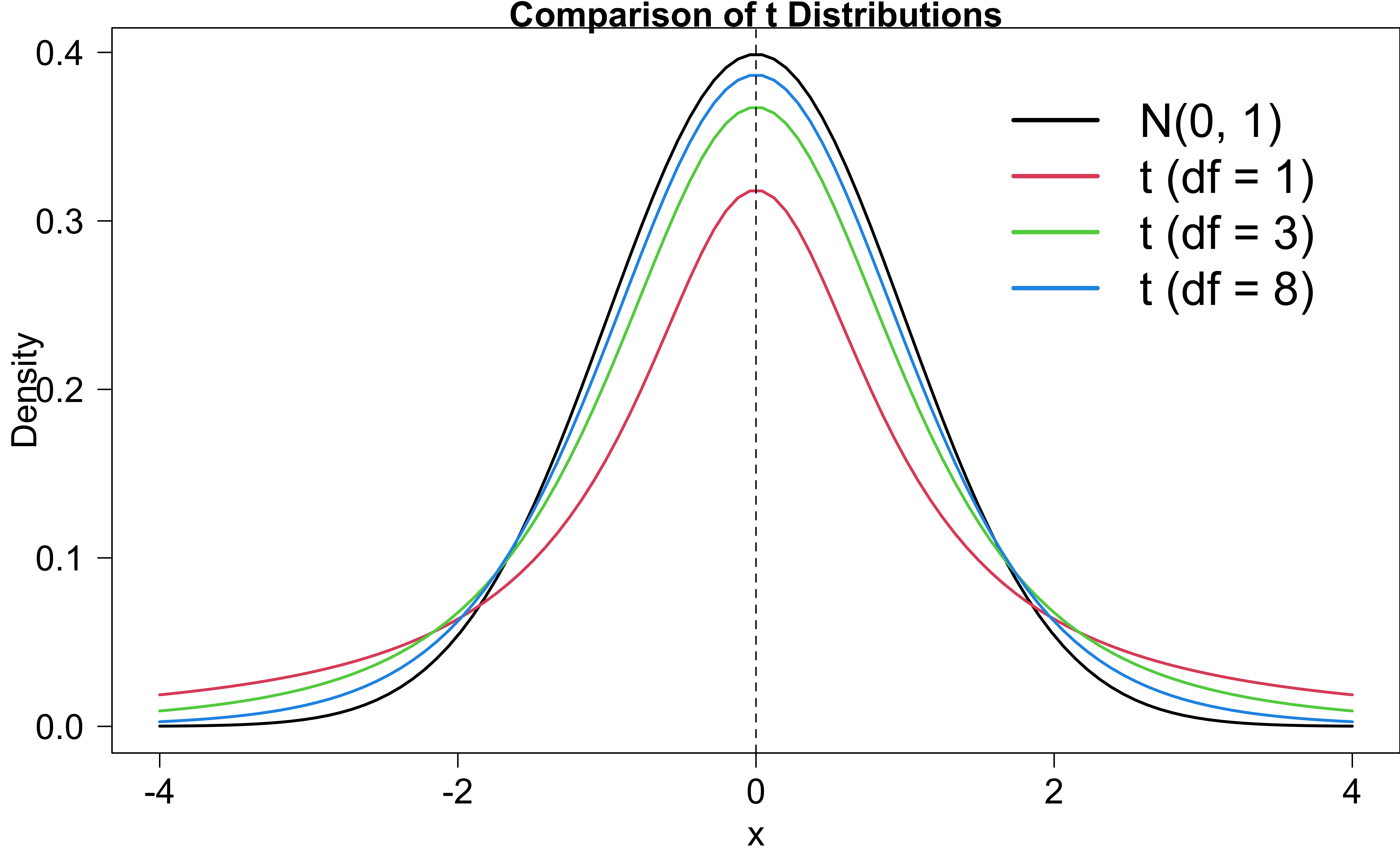
• Symmetric about the mean 0 and bell-shaped as \(N(0, 1)\).

• More variability than \(N(0, 1)\) (heavier tails and lower peak).

• The variability is different for different sample sizes (degrees of freedom).

• As \(n \rightarrow \infty\) \((df \rightarrow \infty)\), the Student t distribution approaches to \(N(0, 1)\).

Critical Values of \(t_{\alpha/2, n-1}\)

• When \(\sigma\) is unknown, we use \(t_{\alpha/2, n-1}\) as the critical value, instead of \(z_{\alpha/2}\).

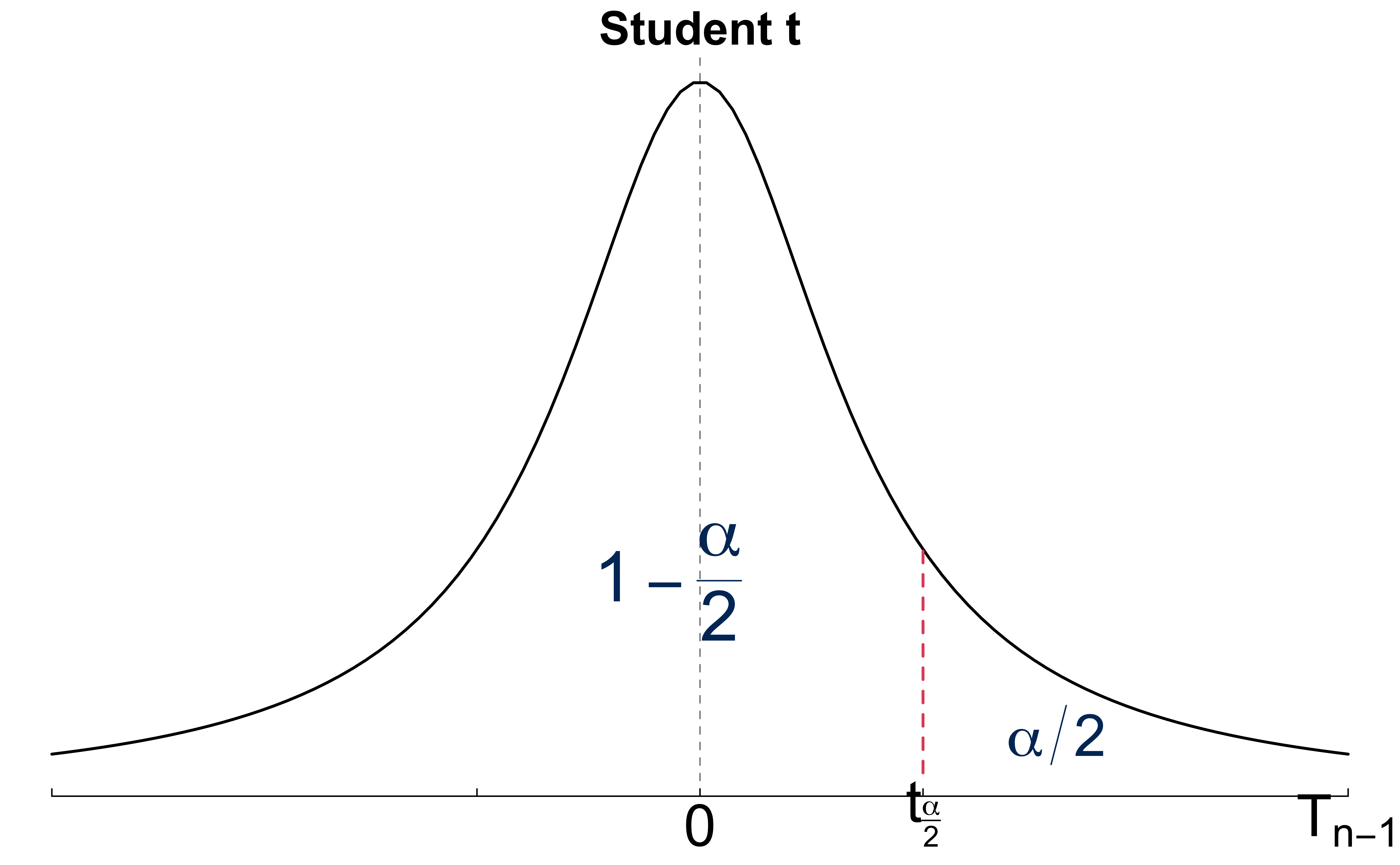
With the same \(\alpha\), \(t_{\alpha, n-1}\) or \(z_{\alpha}\) is larger?

Critical Values of \(t_{\alpha/2, n-1}\)

Given the same confidence level \(1-\alpha\), \(t_{\alpha/2, n-1} > z_{\alpha/2}\).

Level	t df = 5	t df = 15	t df = 30	t df = 1000	t df = inf	z
90%	2.02	1.75	1.70	1.65	1.64	1.64
95%	2.57	2.13	2.04	1.96	1.96	1.96
99%	4.03	2.95	2.75	2.58	2.58	2.58

CI for \(\mu\) When \(\sigma\) is Unknown

• The \((1-\alpha)100\%\) confidence interval for \(\mu\) when \(\sigma\) is unknown is \[\left(\overline{x} - t_{\alpha/2, n-1} \frac{s}{\sqrt{n}}, \overline{x} + t_{\alpha/2, n-1} \frac{s}{\sqrt{n}}\right)\]

• Given the same confidence level \(1-\alpha\), \(t_{\alpha/2, n-1} > z_{\alpha/2}\).

We are more “uncertain” when doing inference about \(\mu\) because we also don’t have information about \(\sigma\), and replacing it with \(s\) adds additional uncertainty.

Computation in R (t interval)

• Back to the systolic blood pressure (SBP) example. We have \(n=16\) and \(\overline{x} = 121.5\).

• Estimate the mean SBP with a 95% confidence interval with unknown \(\sigma\) and \(s = 5\).

alpha <- 0.05
n <- 16
x_bar <- 121.5
s <- 5  ## sigma is unknown and s = 5

## t-critical value
(cri_t <- qt(p = alpha / 2, df = n - 1, lower.tail = FALSE)) 

[1] 2.131

## margin of error
(m_t <- cri_t * (s / sqrt(n)))  

[1] 2.664

## 95% CI for mu when sigma is unknown
x_bar + c(-1, 1) * m_t  

[1] 118.8 124.2

Summary

	Numerical Data, \(\sigma\) known	Numerical Data, \(\sigma\) unknown
Parameter of Interest	Population Mean \(\mu\)	Population Mean \(\mu\)
Confidence Interval	\(\bar{x} \pm z_{\alpha/2} \frac{\sigma}{\sqrt{n}}\)	\(\bar{x} \pm t_{\alpha/2, n-1} \frac{s}{\sqrt{n}}\)

• Remember to check if the population is normally distributed or \(n>30\).

• What if the population is not normal and \(n \le 30\)?

• Use a so-called nonparametric method, for example bootstrapping. (Your project?!)