Statistical Inference: Hypothesis Testing

MATH 4720/MSSC 5720 Introduction to Statistics

Dr. Cheng-Han Yu
Department of Mathematical and Statistical Sciences
Marquette University

Hypothesis Testing

What is a Hypothesis Testing?

• A hypothesis is a claim or statement about a property of a population, often the value of a population parameter.
  • The mean body temperature of humans is less than \(98.6^{\circ}\) F, or \(\mu < 98.6\).
  • Marquette students’ IQ scores has standard deviation equal to 15, or \(\sigma = 15\).

• Null hypothesis \((H_0)\): a statement that the value of a parameter is
  • equal to some claim value
  • the negation of the alternative hypothesis
  • often represents a skeptical perspective to be tested
• Alternative hypothesis \((H_1\) or \(H_a)\): a claim that the parameter is less than, greater than or not equal to some value.
  • usually our research hypothesis of some new scientific theory or finding

• The null hypothesis (H0) often represents either a skeptical perspective or a claim to be tested.
• The alternative hypothesis (HA) is an alternative claim and is often represented by a range of possible parameter values.
• The null hypothesis often represents a skeptical position or a perspective of “no difference”.
• The alternative hypothesis generally represents a new or stronger perspective.

Null and Alternative Hypothesis

A \(H_0\) claim or \(H_1\) claim?

• The percentage of Marquette female students loving Japanese food is equal to 80%.

• On average, Marquette students consume less than 3 drinks per week.

• A hypothesis testing ¹ is a procedure to decide whether to reject \(H_0\) or not by how much evidence against \(H_0\).

A hypothesis testing is a method for calculating the probability of making a specific observation under a working hypothesis, called the null hypothesis.

1. Null Hypothesis Statistical Testing (NHST), statistical testing or test of significance.

Hypothesis Testing Example

A person is charged with a crime.

• A jury decide whether the person is guilty or not.

• The accuse is assumed to be innocent until the jury declares otherwise.

• Only if overwhelming evidence of the person’s guilt can be shown is the jury expected to declare the person guilty, otherwise the person is considered not guilty.

What should be \(H_0\) and \(H_a\)?

• A person comes into court charged with a crime.

• A jury decide whether the person is guilty or not.

• Even though the person is charged with the crime, at the beginning of the trial (and until the jury declares otherwise) the accuse is assumed to be innocent.

• Only if overwhelming evidence of the person’s guilt can be shown is the jury expected to declare the person guilty, otherwise the person is considered innocent.

.question[ What should be \(H_0\) and \(H_a\)?]

• \(H_0:\) The person is not guilty 🙂

• \(H_1:\) The person is guilty 😟

• Evidence: Photos, videos, witness, fingerprint, DNA

• Decision Rule: Jury’s voting

• Conclusion: Verdict “guilty” or “NOT enough evidence to convict”

How to Formally Do a Statistical Hypothesis Testing

• Step 0: Check Method Assumptions

• Step 1: Set the \(H_0\) and \(H_a\) in Symbolic Form from a Claim

• Step 2: Set the Significance Level \(\alpha\)

• Step 3: Calculate the Test Statistic (Evidence)

(Decision Rule I: Critical Value Method)

• Step 4-c: Find the Critical Value

• Step 5-c: Draw a Conclusion Using Critical Value Method

(Decision Rule II: P-Value Method)

• Step 4-p: Find the P-Value

• Step 5-p: Draw a Conclusion Using P-Value Method

• Step 6: Restate the Conclusion in Nontechnical Terms, and Address the Original Claim

• 😎 No worries, we will learn the steps step by step!

The New Treatment is Effective?

• A population of hypertension group is normal and has mean blood pressure (BP) 150.

• After 6 months of treatment, BP was recorded on 25 patients of this population, and \(\overline{x} = 147.2\) and \(s = 5.5\).

• Goal: Determine whether a new treatment is effective in reducing BP.

Step 0: Check Method Assumptions

The testing methods are based on normality or approximate normality by CLT.

• Random sample

• Normally distributed and/or \(n > 30\)

The New Treatment is Effective?

• A population of hypertension group is normal and has mean blood pressure (BP) 150.

• After 6 months of treatment, BP was recorded on 25 patients of this population, and \(\overline{x} = 147.2\) and \(s = 5.5\).

• Goal: Determine whether a new treatment is effective in reducing BP.

Step 1: Set the \(H_0\) and \(H_1\) from a Claim

• 👩‍🏫 The mean IQ score of statistics professors is higher than 120.

• \(\begin{align}&H_0: \mu \le 120 \\ &H_1: \mu > 120 \end{align}\)

• 💵 The mean starting salary for Marquette graduates who didn’t take MATH 4720 is less than $60,000.

• \(\begin{align} &H_0: \mu \ge 60000 \\ &H_1: \mu < 60000 \end{align}\)

• 📺 The mean time between uses of a TV remote control by males during commercials equals 5 sec.

• \(\begin{align} &H_0: \mu = 5 \\ &H_1: \mu \ne 5 \end{align}\)

( \(H_0\) claim)

The New Treatment is Effective?

• A population of hypertension group is normal and has mean blood pressure (BP) 150.

• After 6 months of treatment, BP was recorded on 25 patients of this population, and \(\overline{x} = 147.2\) and \(s = 5.5\).

• Goal: Determine whether a new treatment is effective in reducing BP .

• The claim that the new treatment is effective in reducing BP means the mean BP is less than 150. ( \(H_1\) claim )

• \(\small \begin{align} &H_0: \mu = 150 \\ &H_1: \mu < 150 \end{align}\)

Step 2: Set the Significance Level \(\alpha\)

• The significant level \(\alpha\) determines how rare or unlikely our evidence must be in order to represent sufficient evidence against \(H_0\).

• An \(\alpha\) level of 0.05 implies that evidence occurring with probability lower than 5% will be considered sufficient evidence against \(H_0\) (Reject \(H_0\)).

• \(\alpha = P(\text{Reject } H_0 \mid H_0 \text{ is true})\)

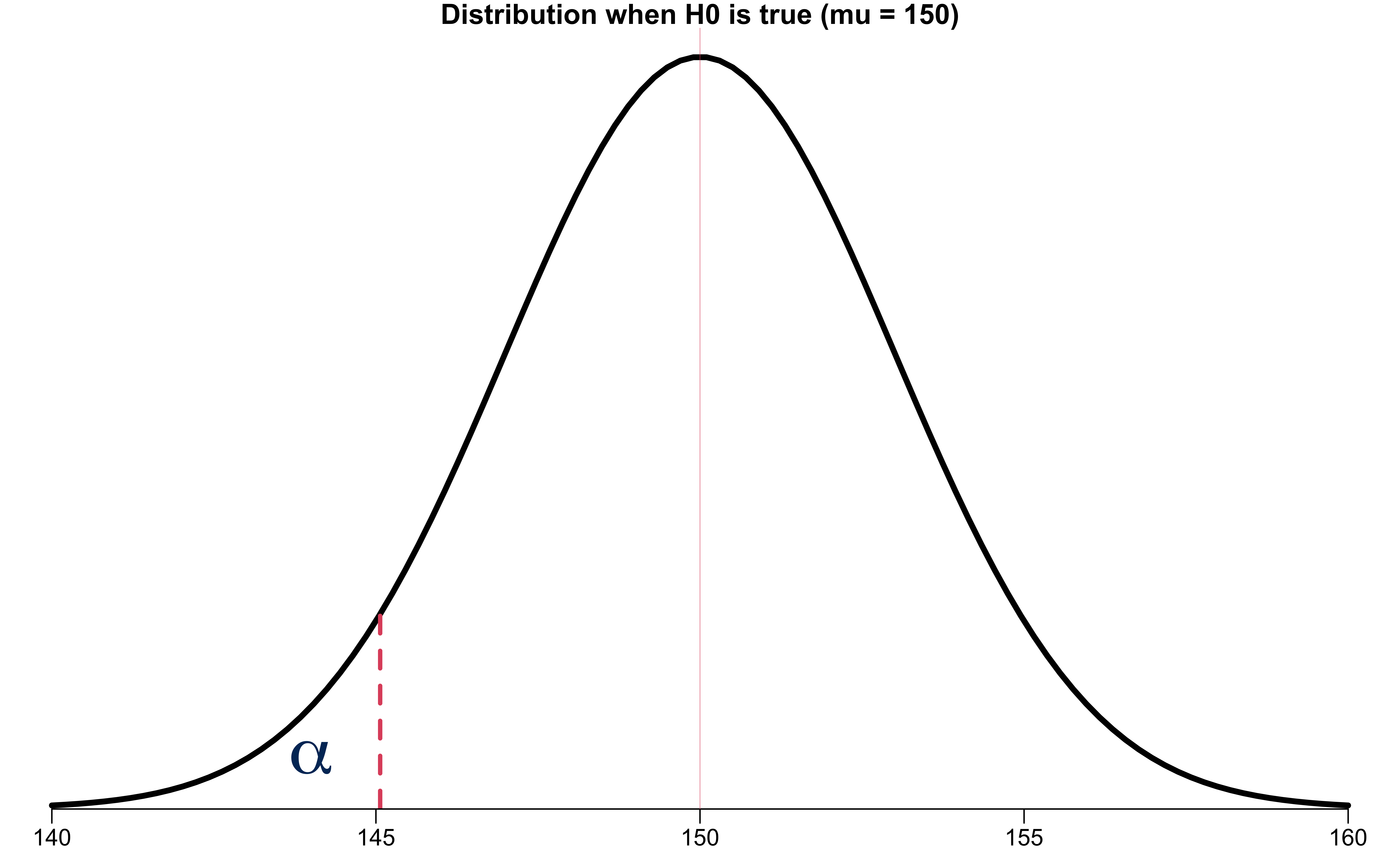
Rare Event Rule: If, under a given assumption, the probability of a particular observed event is exceptional small, we conclude that the assumption is probably not correct.

• \(\alpha\) is like a threshold. If our collected evidence has a smaller probability than \(\alpha\) happening, then the current assumption or claim is probably not correct.
• If the true mean IQ of statistics professors is 120, \(\alpha \%\) of them will have IQ greater than 125.
• The level \(\alpha\) is related to \(\alpha\) used in confidence intervals for defining a “critical value”.
• \(\alpha = 0.05\) means that we incorrectly reject \(H_0\) 5 out of every 100 times we collect a sample and run the test.

The New Treatment is Effective?

• A population of hypertension group is normal and has mean blood pressure (BP) 150.

• After 6 months of treatment, BP was recorded on 25 patients of this population, and \(\overline{x} = 147.2\) and \(s = 5.5\).

• Goal: Determine whether a new treatment is effective in reducing BP.

• \(\small \begin{align} &H_0: \mu = 150 \\ &H_1: \mu < 150 \end{align}\)

• Set \(\alpha= 0.05\). We are asking: Is there a sufficient evidence at \(\alpha= 0.05\) that the new treatment is effective?

Step 3: Calculate the Test Statistic

• A test statistic is a statistic value used in making a decision about the \(H_0\).

• Suppose \(H_0: \mu = \mu_0 \quad H_1: \mu < \mu_0\)

• When computing a test statistic, we assume \(H_0\) is true.

• When \(\sigma\) is known, the test statistic for testings about \(\mu\) is

\[\small \boxed{ z_{test} = \frac{\overline{x} - \color{blue}{\mu_0}}{\sigma/\sqrt{n}} }\]

Guess what test statistic we use when \(\sigma\) is unknown!

• When \(\sigma\) is unknown, the test statistic for testings about \(\mu\) is

\[\small \boxed{ t_{test} = \frac{\overline{x} - \color{blue}{\mu_0}}{s/\sqrt{n}} }\]

The New Treatment is Effective?

• A population of hypertension group is normal and has mean blood pressure (BP) 150.

• After 6 months of treatment, BP was recorded on 25 patients of this population, \(\overline{x} = 147.2\) and \(s = 5.5\) .

• Goal: Determine whether a new treatment is effective in reducing BP.

• \(\small \begin{align} &H_0: \mu = 150 \\ &H_1: \mu < 150 \end{align}\)

• The test statistic is \(\small t_{test} = \frac{\overline{x} - \mu_0}{s/\sqrt{n}} = \frac{147.2 - 150}{5.5/\sqrt{25}} = -2.55\)

Step 4-c: Find the Critical Value

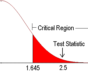
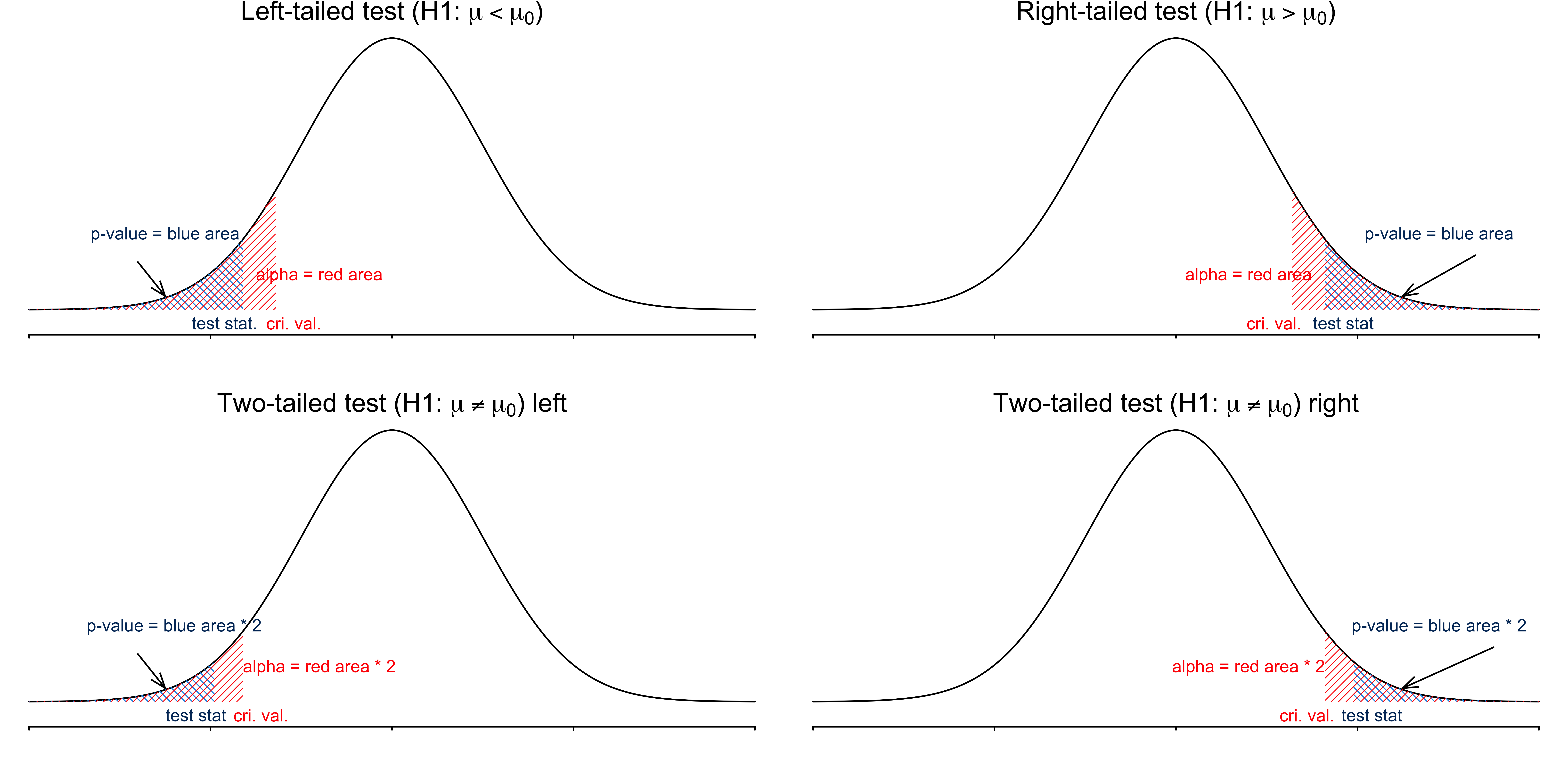
• The critical value(s) separates the rejection region or critical region (where we reject \(H_0\)) from the values of the test statistic that do not lead to rejection of \(H_0\).
  • They depends on whether the test is right-tailed, left-tailed or two-tailed.

In the absence of prior evidence that people typically wish to be lighter (or heavier), it is reasonable to begin with an alternative hypothesis that allows for differences in either direction. A one-sided alternative could be used if, for example, an investigator felt there was prior evidence that people typically wish to weigh less than they currently do:

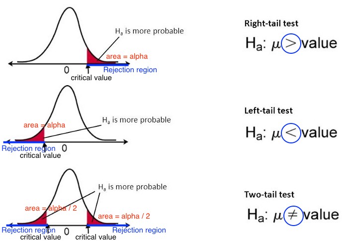
Step 4-c: Find the Critical Value

• 👉 \(z_{\alpha}\) is such that \(P(Z > z_{\alpha}) = \alpha\) and \(Z \sim N(0, 1)\).

• 👉 \(t_{\alpha, n-1}\) is such that \(P(T > t_{\alpha, n-1}) = \alpha\) and \(T \sim t_{n-1}\).

Condition	Right-tailed \((H_1: \mu > \mu_0)\)	Left-tailed \((H_1: \mu < \mu_0)\)	Two-tailed \((H_1: \mu \ne \mu_0)\)
\(\sigma\) known	\(z_{\alpha}\)	\(-z_{\alpha}\)	\(-z_{\alpha/2}\) and \(z_{\alpha/2}\)
\(\sigma\) unknown	\(t_{\alpha, n-1}\)	\(-t_{\alpha, n-1}\)	\(-t_{\alpha/2, n-1}\) and \(t_{\alpha/2, n-1}\)

• \(z_{0.025} =\) 1.96, \(z_{0.05} =\) 1.64

• \(z_{\alpha}\) and \(t_{\alpha, n-1}\) are always positive.

The New Treatment is Effective?

• A population of hypertension group is normal and has mean blood pressure (BP) 150.

• After 6 months of treatment, BP was recorded on 25 patients of this population, \(\overline{x} = 147.2\) and \(s = 5.5\) .

• Goal: Determine whether a new treatment is effective in reducing BP.

• \(\small \begin{align} &H_0: \mu = 150 \\ &H_1: \mu < 150 \end{align}\)

• The test statistic is \(\small t_{test} = \frac{\overline{x} - \mu_0}{s/\sqrt{n}} = \frac{147.2 - 150}{5.5/\sqrt{25}} = -2.55\)

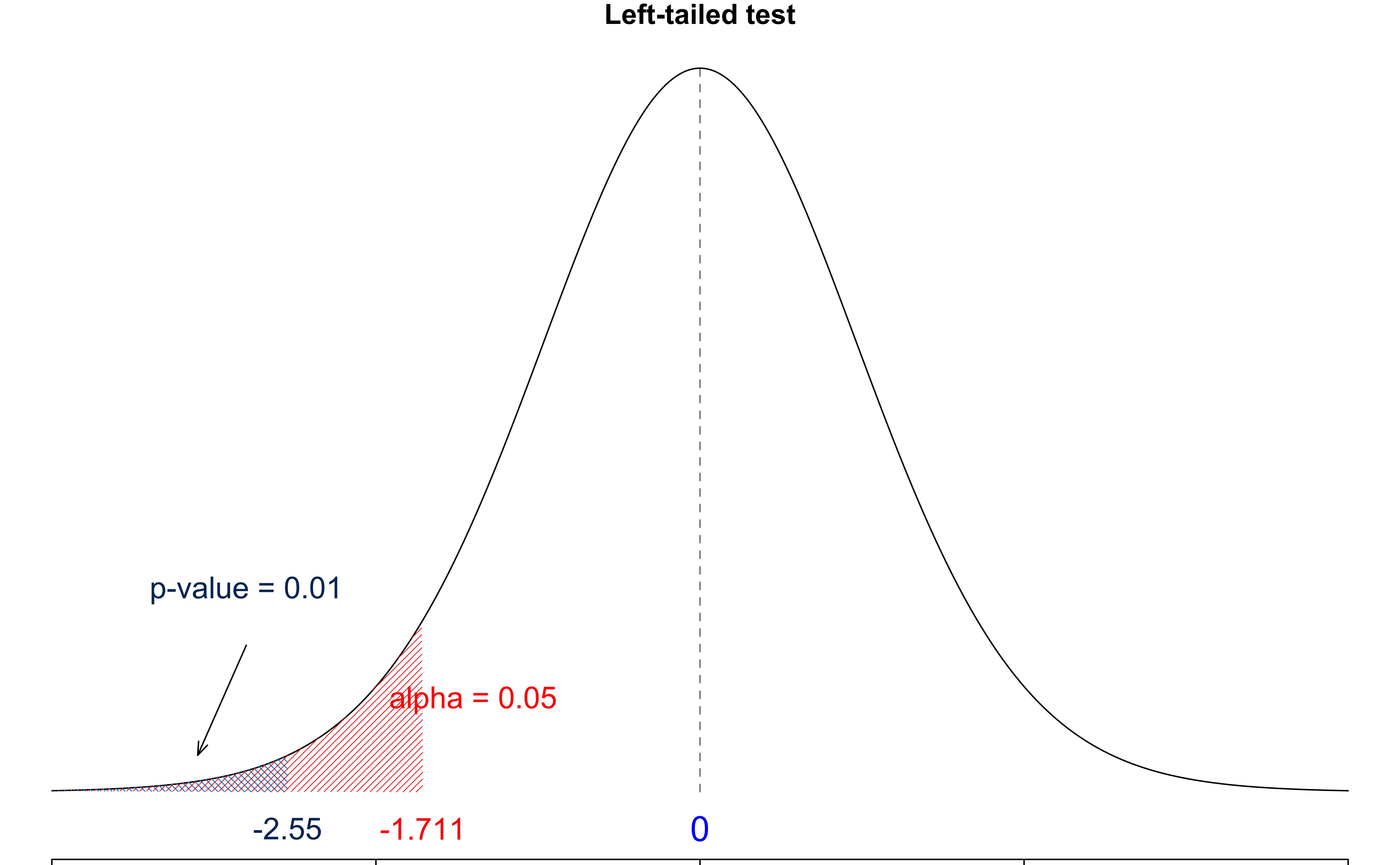
• The critical value is \(\small -t_{0.05, 25-1} = -t_{0.05, 24} = -1.711\)

Step 5-c: Draw a Conclusion Using Critical Value

If the test statistic is

• in the rejection region, we reject \(H_0\).

• not in the rejection region, we do not or fail to reject \(H_0\).

Reject \(H_0\) if

Condition	Right-tailed \((H_1: \mu > \mu_0)\)	Left-tailed \((H_1: \mu < \mu_0)\)	Two-tailed \((H_1: \mu \ne \mu_0)\)
\(\sigma\) known	\(z_{test} > z_{\alpha}\)	\(z_{test} < -z_{\alpha}\)	\(\mid z_{test}\mid \, > z_{\alpha/2}\)
\(\sigma\) unknown	\(t_{test} > t_{\alpha, n-1}\)	\(t_{test} < -t_{\alpha, n-1}\)	\(\mid t_{test}\mid \, > t_{\alpha/2, n-1}\)

\(|z_{test}| > z_{\alpha/2}\)
\(|t_{test}| > t_{\alpha/2, n-1}\)

The New Treatment is Effective?

• A population of hypertension group is normal and has mean blood pressure (BP) 150.

• After 6 months of treatment, BP was recorded on 25 patients of this population, \(\overline{x} = 147.2\) and \(s = 5.5\) .

• Goal: Determine whether a new treatment is effective in reducing BP.

• \(\small \begin{align} &H_0: \mu = 150 \\ &H_1: \mu < 150 \end{align}\)

• The test statistic is \(\small t_{test} = \frac{\overline{x} - \mu_0}{s/\sqrt{n}} = \frac{147.2 - 150}{5.5/\sqrt{25}} = -2.55\)

• The critical value is \(\small -t_{0.05, 25-1} = -t_{0.05, 24} = -1.711\)

• We reject \(H_0\) if \(t_{test} < -t_{\alpha, n-1}\). Since \(\small t_{test} = -2.55 < -1.711 = -t_{\alpha, n-1}\), we reject \(H_0\).

Step 4-p: Find the P-Value

• The \(p\)-value measures the strength of the evidence against \(H_0\) provided by the data.

• The smaller the \(p\)-value, the greater the evidence against \(H_0\).

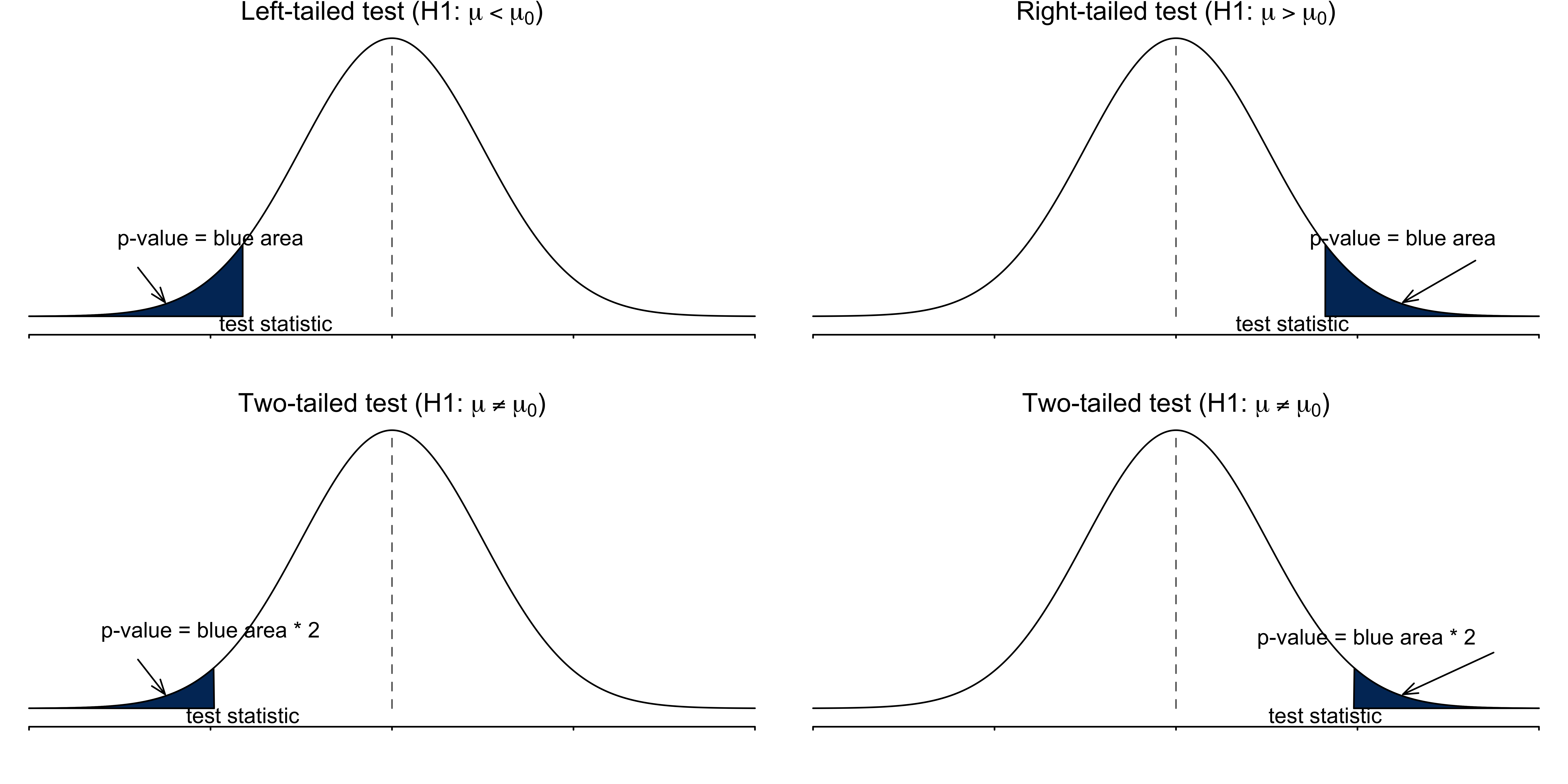
• The \(p\)-value is the probability of getting a test statistic value that is at least as extreme as the one obtained from the data, assuming that \(H_0\) is true. \((\mu = \mu_0)\)

  • For example, \(p\)-value \(= P(Z \ge z_{test} \mid H_0)\) for a right-tailed test.

• What is the chance of having evidence that is more unlikely to happen than our current collected evidence?

P-Value Illustration

The New Treatment is Effective?

• A population of hypertension group is normal and has mean blood pressure (BP) 150.

• After 6 months of treatment, BP was recorded on 25 patients of this population, \(\overline{x} = 147.2\) and \(s = 5.5\) .

• Goal: Determine whether a new treatment is effective in reducing BP.

• \(\small \begin{align} &H_0: \mu = 150 \\ &H_1: \mu < 150 \end{align}\)

• This is a left-tailed test, so the \(p\)-value is \(P(T < t_{test})=P(T < -2.55) =\) 0.01

• Step 5-p: We reject \(H_0\) if \(p\)-value < \(\alpha\). Since \(p\)-value \(= 0.0088 < 0.05 = \alpha\), we reject \(H_0\).
• Step 6: There is sufficient evidence to support the claim that the new treatment is effective.

Step 5-p: Draw a Conclusion Using P-Value Method

• If \(p\)-value \(\le \alpha\) , reject \(H_0\).

• If \(p\)-value \(> \alpha\), do not reject \(H_0\).

Condition	Right-tailed \((H_1: \mu > \mu_0)\)	Left-tailed \((H_1: \mu < \mu_0)\)	Two-tailed \((H_1: \mu \ne \mu_0)\)
\(\sigma\) known	\(P(Z > z_{test} \mid H_0)\)	\(P(Z < z_{test} \mid H_0)\)	\(2P(Z > \,\mid z_{test} \mid \, \mid H_0)\)
\(\sigma\) unknown	\(P(T > t_{test} \mid H_0)\)	\(P(T < t_{test} \mid H_0)\)	\(2P(T > \, \mid t_{test} \mid \, \mid H_0)\)

\(2P(Z > z_{test} \mid H_0)\) if \(z_{test}\) on the right
\(2P(Z < z_{test} \mid H_0)\) if \(z_{test}\) on the left \(2P(T > t_{test} \mid H_0)\) if \(t_{test}\) on the right
\(2P(T < t_{test} \mid H_0)\) if \(t_{test}\) on the left

The New Treatment is Effective?

• A population of hypertension group is normal and has mean blood pressure (BP) 150.

• After 6 months of treatment, BP was recorded on 25 patients of this population, \(\overline{x} = 147.2\) and \(s = 5.5\) .

• Goal: Determine whether a new treatment is effective in reducing BP.

• \(\small \begin{align} &H_0: \mu = 150 \\ &H_1: \mu < 150 \end{align}\)

• This is a left-tailed test, so the \(p\)-value is \(P(T < t_{test})=P(T < -2.55) =\) 0.01

• We reject \(H_0\) if \(p\)-value < \(\alpha\). Since \(p\)-value \(= 0.01 < 0.05 = \alpha\), we reject \(H_0\).

• Step 6: There is sufficient evidence to support the claim that the new treatment is effective.

Both Methods Lead to the Same Conclusion

Step 6: Restate the Conclusion in Nontechnical Terms, and Address the Original Claim

https://www.drdawnwright.com/category/statistics/

https://www.pinterest.com/pin/287878601159173631/

Note! Why can’t we say we “accept the null”? The reason is that we are assuming the null hypothesis is true and trying to see if there is evidence against it. Therefore, the conclusion should be in terms of rejecting the null.

The New Treatment is Effective?

• A population of hypertension group is normal and has mean blood pressure (BP) 150.

• After 6 months of treatment, BP was recorded on 25 patients of this population, \(\overline{x} = 147.2\) and \(s = 5.5\) .

• Goal: Determine whether a new treatment is effective in reducing BP.

• \(\small \begin{align} &H_0: \mu = 150 \\ &H_1: \mu < 150 \end{align}\)

• There is sufficient evidence to support the claim that the new treatment is effective.

Example Calculation in R

## create objects for any information we have
alpha <- 0.05; mu_0 <- 150; 
x_bar <- 147.2; s <- 5.5; n <- 25

## Test statistic
(t_test <- (x_bar - mu_0) / (s / sqrt(n))) 

[1] -2.545

## Critical value
(t_cri <- qt(alpha, df = n - 1, lower.tail = TRUE)) 

[1] -1.711

## p-value
(p_val <- pt(t_test, df = n - 1, lower.tail = TRUE)) 

[1] 0.008878

[1] "Reject H0 by crit. value"

[1] "Reject H0 by p-value"

Example 2: Two-tailed z-test

The milk price of a gallon of 2% milk is normally distributed with standard deviation of $0.10.

• Last week the mean milk price was 2.78. This week, based on a sample of size 25, the sample mean milk price \(\overline{x} = 2.80\).

• Under \(\alpha = 0.05\), determine if this week the mean price is different.

• Step 1: This is a \(H_1\) claim \(\small \begin{align}&H_0: \mu = 2.78 \\ &H_1: \mu \ne 2.78 \end{align}\)

• Step 2: \(\small \alpha = 0.05\)

• Step 3: \(\small z_{test} = \frac{\overline{x} - \mu_0}{\sigma/\sqrt{n}} = \frac{2.8 - 2.78}{0.1/\sqrt{25}} = 1.00\)

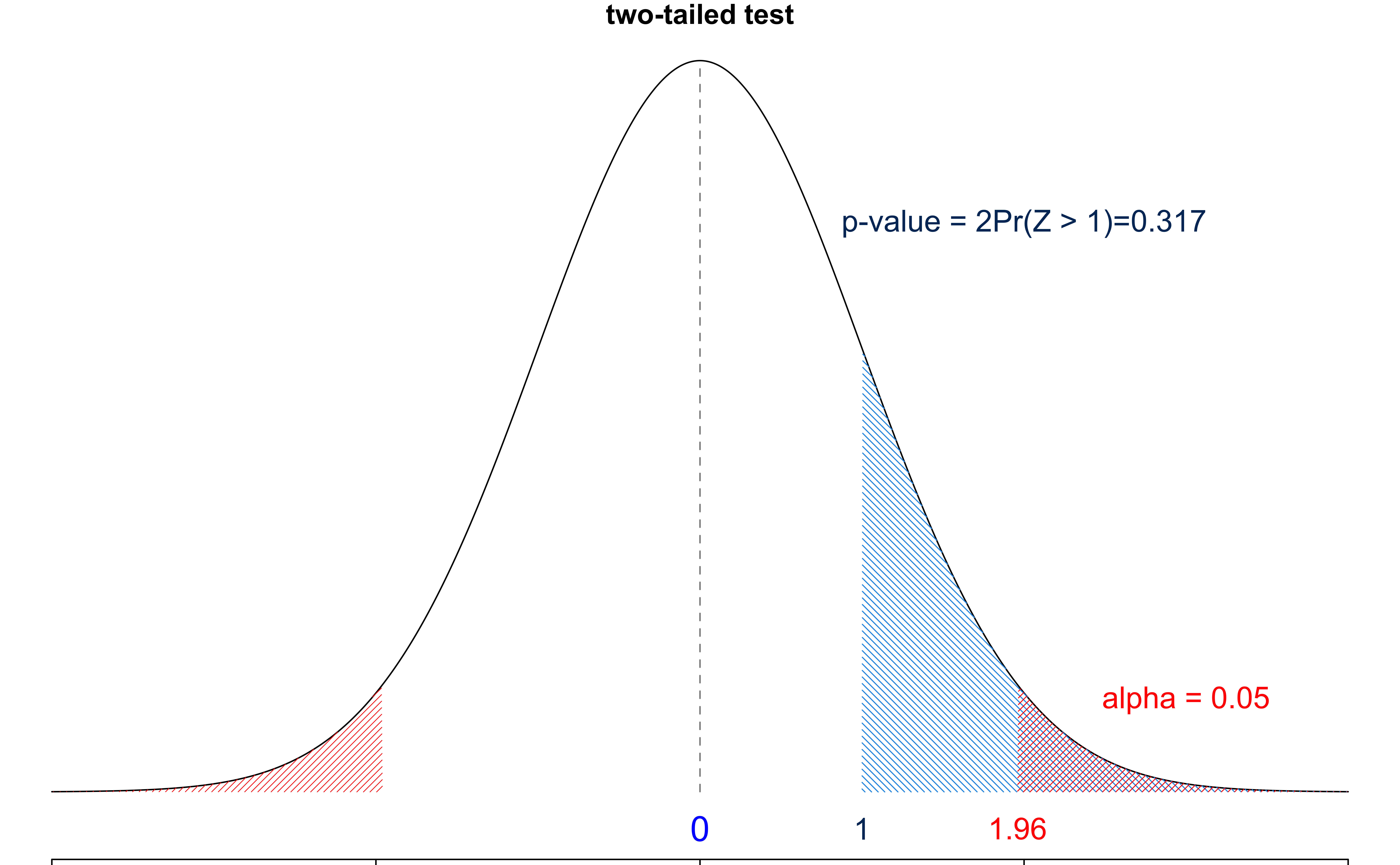
• Step 4-c: \(\small z_{0.05/2} = 1.96\).

• Step 5-c: This is a two-tailed test and we reject \(H_0\) if \(|z_{test}| > z_{\alpha/2}\). Since \(\small |z_{test}| = 1 < 1.96 = z_{\alpha/2}\), we DO NOT reject \(H_0\).

Example 2: two-tailed z-test Cont’d

• Step 4-p: This is a two-tailed test, and the test statistic is on the right \((> 0)\), so the \(p\)-value is \(2P(Z > z_{test})=\) 0.317

• Step 5-p: We reject \(H_0\) if \(p\)-value < \(\alpha\). Since \(p\)-value \(= 0.317 > 0.05 = \alpha\), we DO NOT reject \(H_0\).

• Step 6: There is insufficient evidence to support the claim that this week the mean milk price is different from the price last week.

Example 2 Calculation in R

## create objects to be used
alpha <- 0.05; mu_0 <- 2.78; 
x_bar <- 2.8; sigma <- 0.1; n <- 25

## Test statistic
(z_test <- (x_bar - mu_0) / (sigma / sqrt(n))) 

[1] 1

## Critical value
(z_crit <- qnorm(alpha/2, lower.tail = FALSE)) 

[1] 1.96

## p-value
(p_val <- 2 * pnorm(z_test, lower.tail = FALSE)) 

[1] 0.3173

[1] "Do not reject H0 by critical value method"

[1] "Do not reject H0 by p-value method"

Testing Summary

	Numerical Data, \(\sigma\) known	Numerical Data, \(\sigma\) unknown
Parameter of Interest	Population Mean \(\mu\)	Population Mean \(\mu\)
Test Type	One sample \(\color{blue}{z}\) test \(H_0: \mu = \mu_0\)	One sample \(\color{blue}{t}\) test \(H_0: \mu = \mu_0\)
Confidence Interval	\(\bar{x} \pm z_{\alpha/2} \frac{\sigma}{\sqrt{n}}\)	\(\bar{x} \pm t_{\alpha/2, n-1} \frac{\color{blue}{s}}{\sqrt{n}}\)
Test Stat under \(H_0\)	\(z_{test} = \frac{\overline{x} - \mu_0}{\frac{\sigma}{\sqrt{n}}}\)	\(t_{test} = \frac{\overline{x} - \mu_0}{\frac{\color{blue}{s}}{\sqrt{n}}}\)
\(p\)-value under \(H_0\)	\(H_1: \mu < \mu_0\) \(p\)-value \(=P(Z \le z_{test})\)	\(H_1: \mu < \mu_0\) \(p\)-value \(=P(T_{n-1} \le t_{test})\)
	\(H_1: \mu > \mu_0\) \(p\)-value \(=P(Z \ge z_{test})\)	\(H_1: \mu < \mu_0\) \(p\)-value \(=P(T_{n-1} \ge t_{test})\)
	\(H_1: \mu \ne \mu_0\) \(p\)-value \(=2P(Z \ge \, \mid z_{test}\mid)\)	\(H_1: \mu \ne \mu_0\) \(p\)-value \(=2P(T_{n-1} \ge \, \mid t_{test} \mid)\)

Type I and Type II Errors

Decision	\(H_0\) is true	\(H_0\) is false
Reject \(H_0\)	Type I error	Correct decision
Do not reject \(H_0\)	Correct decision	Type II error

Back to the crime example: \(H_0:\) The person is not guilty v.s. \(H_1:\) The person is guilty

Decision	Truth is the person innocent	Truth is the person guilty
Jury decides the person guilty	Type I error	Correct decision
Jury decides the person innocent	Correct decision	Type II error

• In practice, we will not know for certain if we made the correct decision or if we made one of these two errors.

Type I and Type II Errors

• \(\alpha = P(\text{type I error}) = P(\text{rejecting } H_0 \text{ when } H_0 \text{ is true})\)

• \(\beta = P(\text{type II error}) = P(\text{failing to reject } H_0 \text{ when } H_0 \text{ is false})\)

https://www.statisticssolutions.com/wp-content/uploads/2017/12/rachnovblog.jpg