Inference About Population Variances

MATH 4720/MSSC 5720 Introduction to Statistics

Dr. Cheng-Han Yu
Department of Mathematical and Statistical Sciences
Marquette University

Inference About Population Variances

• One Population Variance

• Comparing Two Population Variances

Inference for One Population Variance

Why Inference for Population Variances?

• We like to know if \(\sigma_1 = \sigma_2\), so a correct or better method can be used.

Which test we learned needs \(\sigma_1 = \sigma_2\)?

In some situations, we care about variation!

• the variation in potency of drugs: affects patients’ health

• the variance of stock prices : the higher the variance, the riskier the investment

• When doing inference for population means,
• We like to know if \(\sigma_1 = \sigma_2\), so that a correct or better method can be used. For example, we use the pooled \(t\)-test if \(\sigma_1 = \sigma_2\) or they are very close to each other for higher power.
• drug for lowering BP. We hope the same amount or dose level of the drug provide the same effect on each individual. We don’t want some patients BP is lowered a lot, but some other patient’s BP is lowered just a little bit.
• We want the new treatment can provide consistent potency and efficacy for all patients.

Inference for Population Variances

• The sample variance \(S^2 = \frac{\sum_{i=1}^n(X_i - \overline{X})^2}{n-1}\) is our point estimator for the population variance \(\sigma^2\).

• The inference for \(\sigma^2\) needs the population to be normal.

❗ The methods can work poorly if the normality is violated, even the sample is large.

• In some situations, we do care about variation.

  • the variation in potency of drugs: affects patients’ health
  • the variance of stock prices : the higher the variance, the riskier the investment

• Intuitively, the sample variance \(S^2 = \frac{\sum_{i=1}^n(X_i - \overline{X})^2}{n-1}\) is our point estimator for the population variance \(\sigma^2\).

• For a random sample of size \(n\) drawn from a population with mean \(\mu\) and variance \(\sigma^2\), \(S^2\) is an unbiased estimator for \(\sigma^2\).

• In Chapter 7, we discuss inference methods for \(\sigma^2\) when the population is assumed normal. The methods discussed here can work poorly if normality is violated, even if the sample is large.

Chi-Squared \(\chi^2\) Distribution

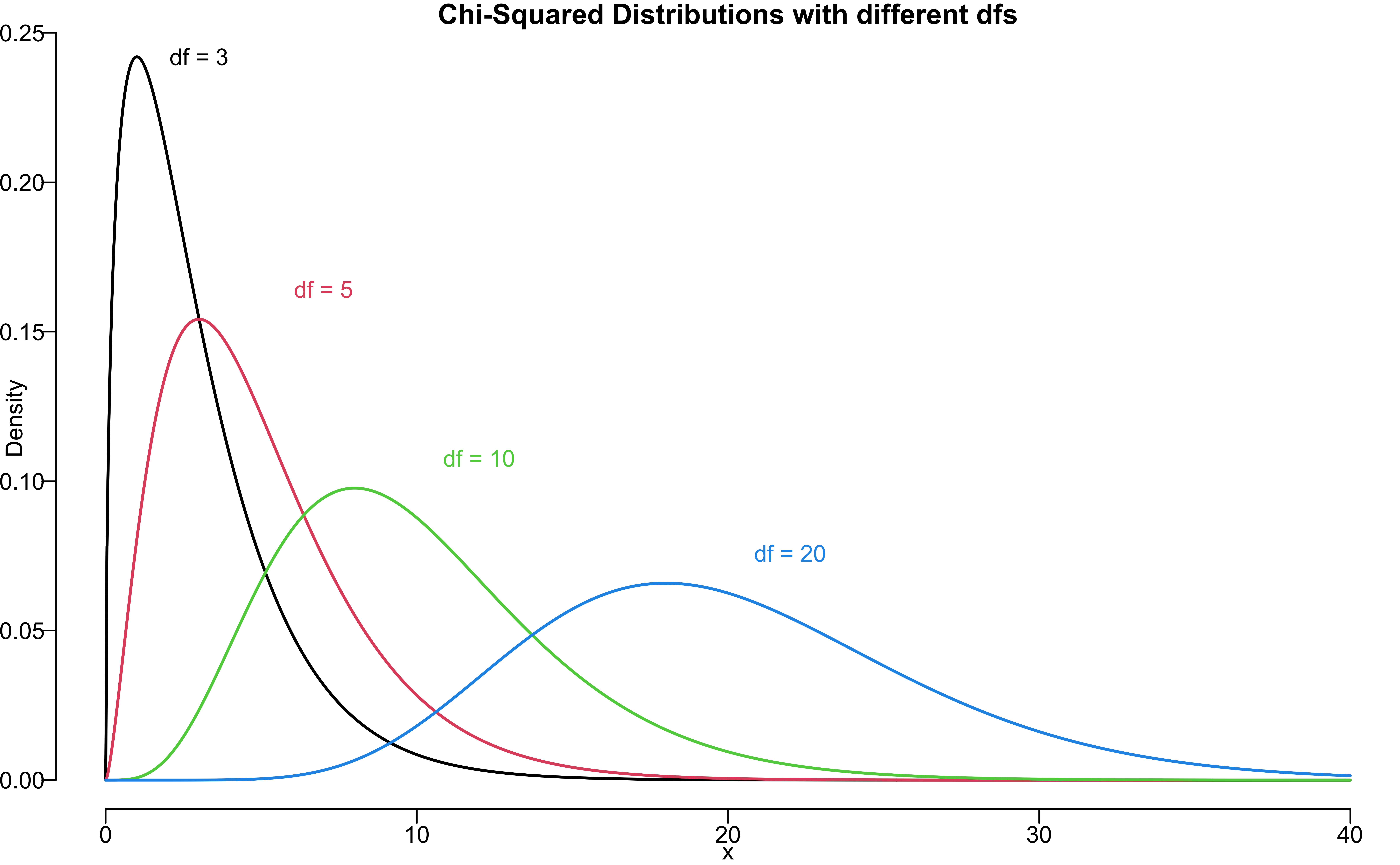
The inference for \(\sigma^2\) involves the \(\chi^2\) distribution.

• Defined over positive numbers

• Parameter: degrees of freedom \(df\)

• Right skewed

• More symmetric as \(df\) gets larger

Upper Tail and Lower Tail of Chi-Square

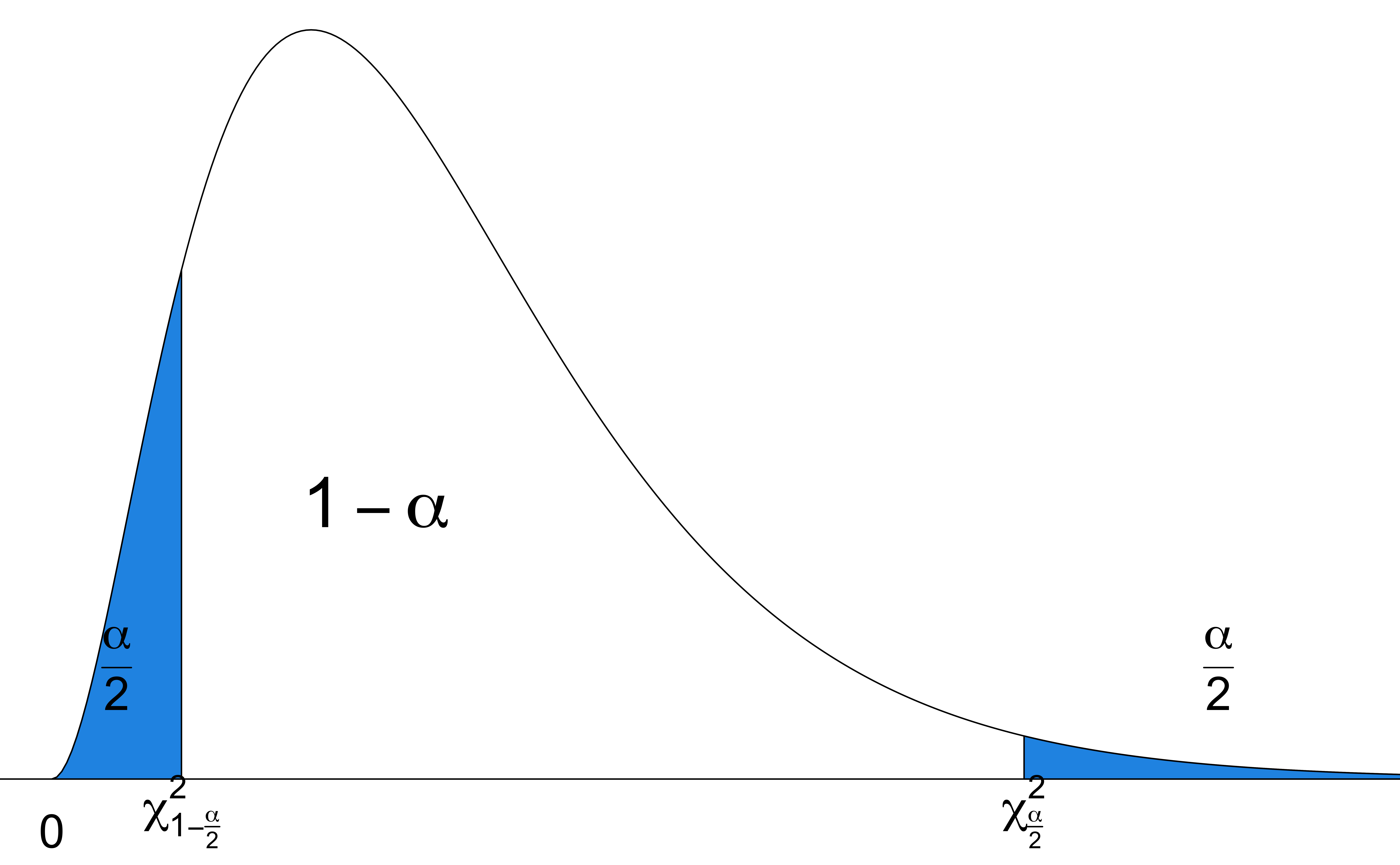
• \(\chi^2_{\frac{\alpha}{2},\, df}\) has area to the right of \(\alpha/2\).

• \(\chi^2_{1-\frac{\alpha}{2},\, df}\) has area to the left of \(\alpha/2\).

• In \(N(0, 1)\), \(z_{1-\frac{\alpha}{2}} = -z_{\frac{\alpha}{2}}\). But \(\chi^2_{1-\frac{\alpha}{2},\,df} \ne -\chi^2_{\frac{\alpha}{2},\,df}\) because of non-symmetry of the \(\chi^2\) distribution.

• Define critical values \(\chi_U^2\) and \(\chi_L^2\).
• When constructing a CI with level \(1-\alpha\), we put \(1-\alpha\) in the middle and

Sampling Distribution

• When a random sample of size \(n\) is from \(\color{red}{N(\mu, \sigma^2)}\), \[ \frac{(n-1)S^2}{\sigma^2} \sim \chi^2_{n-1} \]

• The inference method for \(\sigma^2\) introduced here can work poorly if the normality assumption is violated, even for large samples!

\((1-\alpha)100\%\) Confidence Interval for \(\sigma^2\)

\((1-\alpha)100\%\) CI for \(\sigma^2\) is \[\color{blue}{\left( \frac{(n-1)S^2}{\chi^2_{\frac{\alpha}{2}, \, n-1}}, \frac{(n-1)S^2}{\chi^2_{1-\frac{\alpha}{2}, \, n-1}} \right)}\]

❗ The CI for \(\sigma^2\) cannot be expressed as \((S^2-m, S^2+m)\) anymore!

Example: Supermodel Heights

Listed below are heights (cm) for the simple random sample of 16 female supermodels:

heights <- c(178, 177, 176, 174, 175, 178, 175, 178, 
             178, 177, 180, 176, 180, 178, 180, 176)

• The supermodels’ height is normally distributed.
• Construct a \(95\%\) confidence interval for population standard deviation \(\sigma\).

• \(n = 16\), \(s^2 = 3.4\), \(\alpha = 0.05\).

• \(\chi^2_{\alpha/2, n-1} = \chi^2_{0.025, 15} = 27.49\)

• \(\chi^2_{1-\alpha/2, n-1} = \chi^2_{0.975, 15} = 6.26\)

• The \(95\%\) CI for \(\sigma\) is \(\small \left( \sqrt{\frac{(n-1)s^2}{\chi^2_{\frac{\alpha}{2}, \, n-1}}}, \sqrt{\frac{(n-1)s^2}{\chi^2_{1-\frac{\alpha}{2}, \, n-1}}} \right) = \left( \sqrt{\frac{(16-1)(3.4)}{27.49}}, \sqrt{\frac{(16-1)(3.4)}{6.26}}\right) = (1.36, 2.85)\)

Example: Computation in R

n <- 16
s2 <- var(heights)
al <- 0.05

## two chi-square critical values
chi2_right <- qchisq(al / 2, df = n - 1, lower.tail = FALSE)
chi2_left <- qchisq(al / 2, df = n - 1, lower.tail = TRUE)

## two bounds of CI for sigma2
ci_lwr <- (n - 1) * s2 / chi2_right
ci_upr <- (n - 1) * s2 / chi2_left

## two bounds of CI for sigma
sqrt(ci_lwr)

[1] 1.36

sqrt(ci_upr)

[1] 2.85

Example Cont’d: Testing

Use \(\alpha = 0.05\) to test the claim that “supermodels have heights with a standard deviation that is less than \(\sigma = 7.5\) cm for the population of women”.

• Step 1: \(H_0: \sigma = \sigma_0\) vs. \(H_1: \sigma < \sigma_0\). Here \(\sigma_0 = 7.5\) cm

• Step 2: \(\alpha = 0.05\)

• Step 3: Under \(H_0\), \(\chi_{test}^2 = \frac{(n-1)s^2}{\sigma_0^2} = \frac{(16-1)(3.4)}{7.5^2} = 0.91\), a statistic drawn from \(\chi^2_{n-1}\).

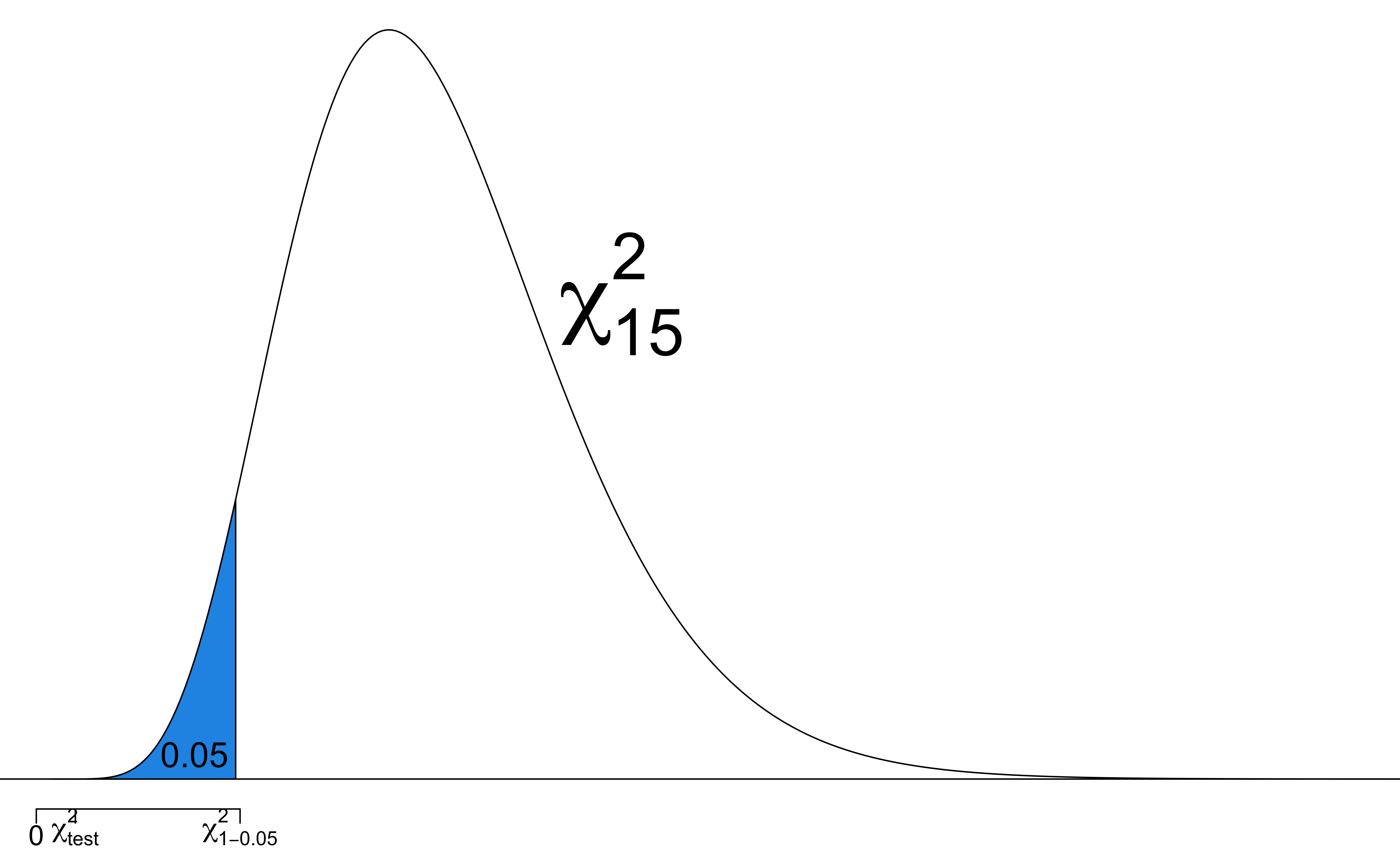
• Step 4-c: This is a left-tailed test. The critical value is \(\chi_{1-\alpha, df}^2 = \chi_{0.95, 15}^2 = 7.26\)
• Step-5-c: Reject \(H_0\) in favor of \(H_1\) if \(\chi_{test}^2 < \chi_{1-\alpha, df}^2\). Since \(0.91 < 7.26\), we reject \(H_0\).

Example Cont’d: Testing

Use \(\alpha = 0.05\) to test the claim that “supermodels have heights with a standard deviation that is less than \(\sigma = 7.5\) cm for the population of women”.

• Step 1: \(H_0: \sigma = \sigma_0\) vs. \(H_1: \sigma < \sigma_0\). Here \(\sigma_0 = 7.5\) cm

• Step 2: \(\alpha = 0.05\)

• Step 3: Under \(H_0\), \(\chi_{test}^2 = \frac{(n-1)s^2}{\sigma_0^2} = \frac{(16-1)(3.4)}{7.5^2} = 0.91\), a statistic drawn from \(\chi^2_{n-1}\).

• Step 6: There is sufficient evidence to support the claim that supermodels have heights with a SD that is less than the SD for the population of women.

Heights of supermodels vary less than heights of women in the general population.

Back to Pooled t-Test

In a pooled t-test, we assume

• both samples are of large size or drawn from a normal population.

• \(\sigma_1 = \sigma_2\)

• Use QQ-plot (and normality tests, Anderson, Shapiro, etc) to check the assumption of normal distribution.

• We learn to check the assumption \(\sigma_1 = \sigma_2\).

• Whenever we use t-statistics, there are assumptions.

Inference for Comparing Two Population Variances

F Distribution

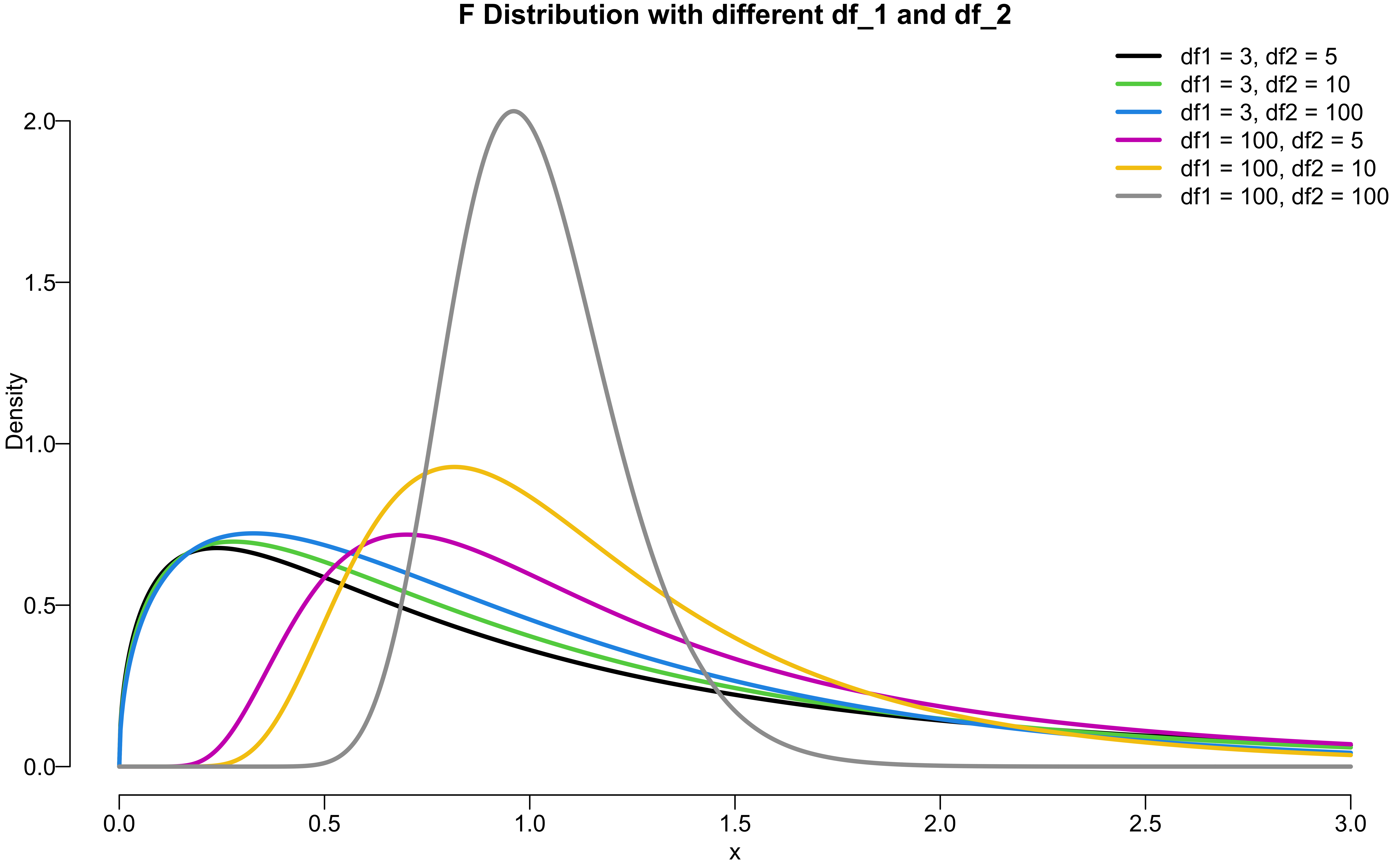
We use \(F\) distribution for the inference about two population variances.

• Two parameters: \(df_1\), \(df_2\)

• Right skewed

• Defined over positive numbers

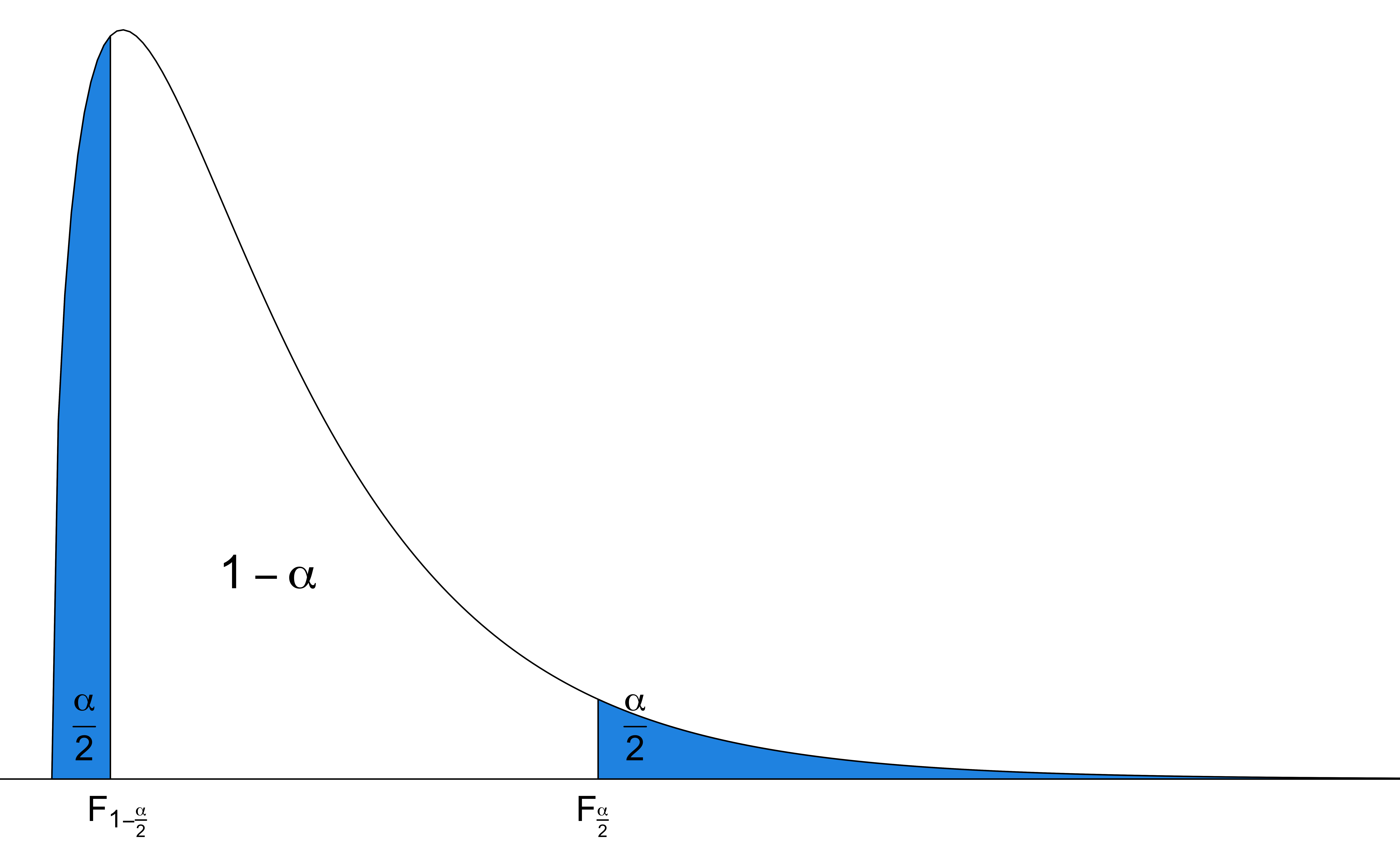
Upper and Lower Tail of F Distribution

• We denote \(F_{\alpha, \, df_1, \, df_2}\) as the \(F\) quantile so that \(P(F_{df_1, df_2} > F_{\alpha, \, df_1, \, df_2}) = \alpha\).

Sampling Distribution

• The random samples of size \(n_1\) and \(n_2\) are independent from two normal populations, \(N(\mu_1, \sigma_1^2)\) and \(N(\mu_2, \sigma_2^2)\).

• The ratio \[\frac{S_1^2/S_2^2}{\sigma_1^2/\sigma_2^2} \sim F_{n_1-1, \, n_2-1}\]

\[\frac{s_1^2/\sigma_1^2}{s_2^2/\sigma_2^2} = \frac{s_1^2/s_2^2}{\sigma_1^2/\sigma_2^2} \sim F_{n_1-1, \, n_2-1}\]

\((1-\alpha)100\%\) Confidence Interval for \(\sigma_1^2 / \sigma_2^2\)

\((1-\alpha)100\%\) CI for \(\sigma_1^2 / \sigma_2^2\) is \[\color{blue}{\left( \frac{s_1^2/s_2^2}{F_{\alpha/2, \, n_1 - 1, \, n_2 - 1}}, \frac{s_1^2/s_2^2}{F_{1-\alpha/2, \, \, n_1 - 1, \, n_2 - 1}} \right)}\]

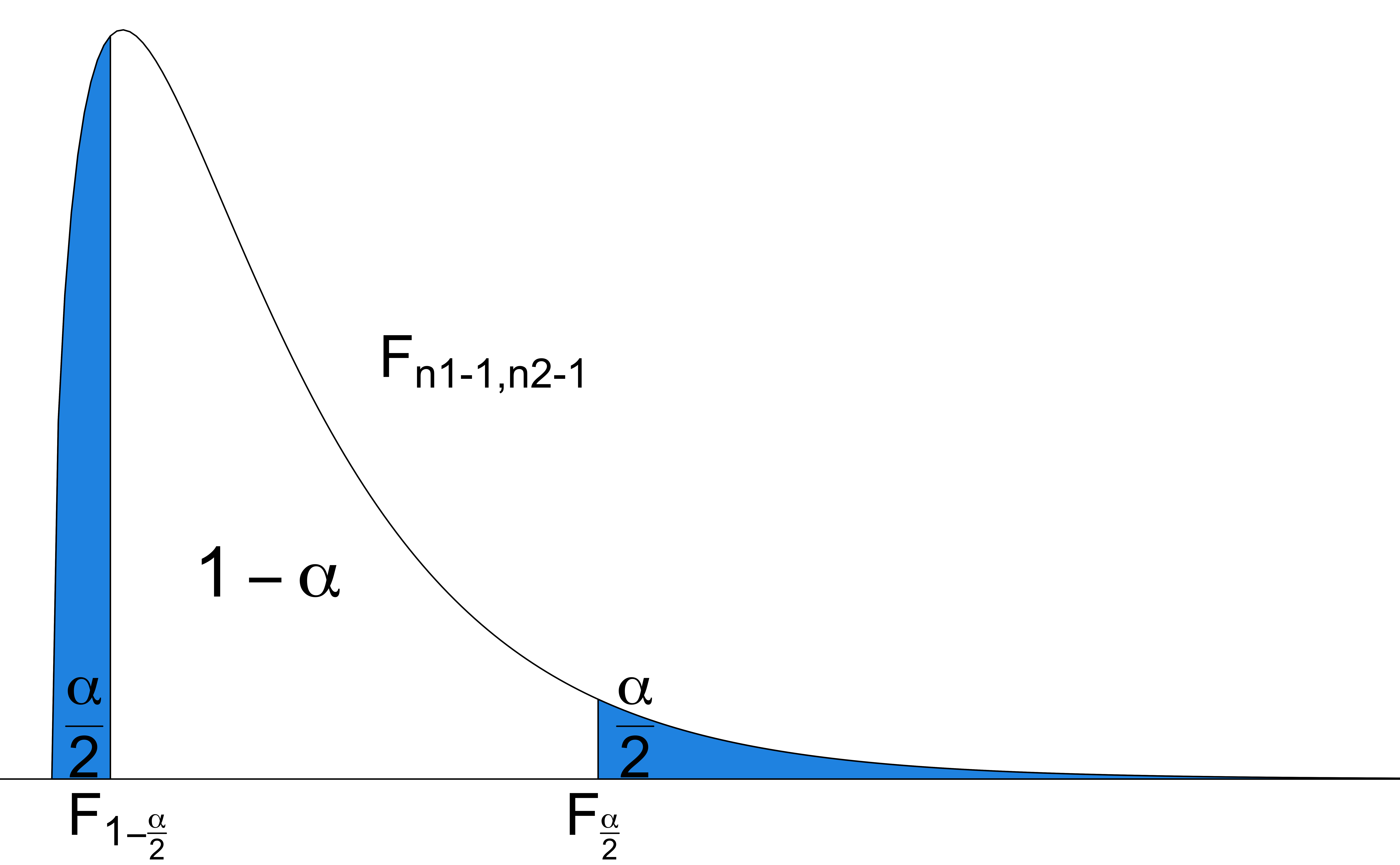
❗ The CI for \(\sigma_1^2 / \sigma_2^2\) cannot be expressed as \(\left(\frac{s_1^2}{s_2^2}-m, \frac{s_1^2}{s_2^2} + m\right)\) anymore!

F test for comparing \(\sigma_1^2\) and \(\sigma_2^2\)

• Step 1: right-tailed \(\small \begin{align} &H_0: \sigma_1 \le \sigma_2 \\ &H_1: \sigma_1 > \sigma_2 \end{align}\) and two-tailed \(\small \begin{align} &H_0: \sigma_1 = \sigma_2 \\ &H_1: \sigma_1 \ne \sigma_2 \end{align}\)

• Step 2: \(\alpha = 0.05\)

• Step 3: Under \(H_0\), \(\sigma_1 = \sigma_2\), and the test statistic is

\[\small F_{test} = \frac{s_1^2/s_2^2}{\sigma_1^2/\sigma_2^2} = \frac{s_1^2}{s_2^2} \sim F_{n_1-1, \, n_2-1}\]

• Step 4-c:
  • Right-tailed: \(F_{\alpha, \, n_1-1, \, n_2-1}\) .
  • Two-tailed: \(F_{\alpha/2, \, n_1-1, \, n_2-1}\) or \(F_{1-\alpha/2, \, n_1-1, \, n_2-1}\)

• Step 5-c:
  • Right-tailed: reject \(H_0\) if \(F_{test} \ge F_{\alpha, \, n_1-1, \, n_2-1}\).
  • Two-tailed: reject \(H_0\) if \(F_{test} \ge F_{\alpha/2, \, n_1-1, \, n_2-1}\) or \(F_{test} \le F_{1-\alpha/2, \, n_1-1, \, n_2-1}\)

Back to the Weight Loss Example

A study was conducted to see the effectiveness of a weight loss program.

• Two groups (Control and Experimental) of 10 subjects were selected.

• The two populations are normally distributed and have the same SD.

• The data on weight loss was collected at the end of six months

  • Control: \(n_1 = 10\), \(\overline{x}_1 = 2.1\, lb\), \(s_1 = 0.5\, lb\)
  • Experimental: \(n_2 = 10\), \(\overline{x}_2 = 4.2\, lb\), \(s_2 = 0.7\, lb\)

• Assumptions:

  • \(\sigma_1 = \sigma_2\)

  • The weight loss for both groups are normally distributed.

Back to the Weight Loss Example: Check if \(\sigma_1 = \sigma_2\)

• \(n_1 = 10\), \(s_1 = 0.5 \, lb\)

• \(n_2 = 10\), \(s_2 = 0.7 \, lb\)

• Step 1: \(\begin{align} &H_0: \sigma_1 = \sigma_2 \\ &H_1: \sigma_1 \ne \sigma_2 \end{align}\)

• Step 2: \(\alpha = 0.05\)

• Step 3: \(F_{test} = \frac{s_1^2}{s_2^2} = \frac{0.5^2}{0.7^2} = 0.51\).

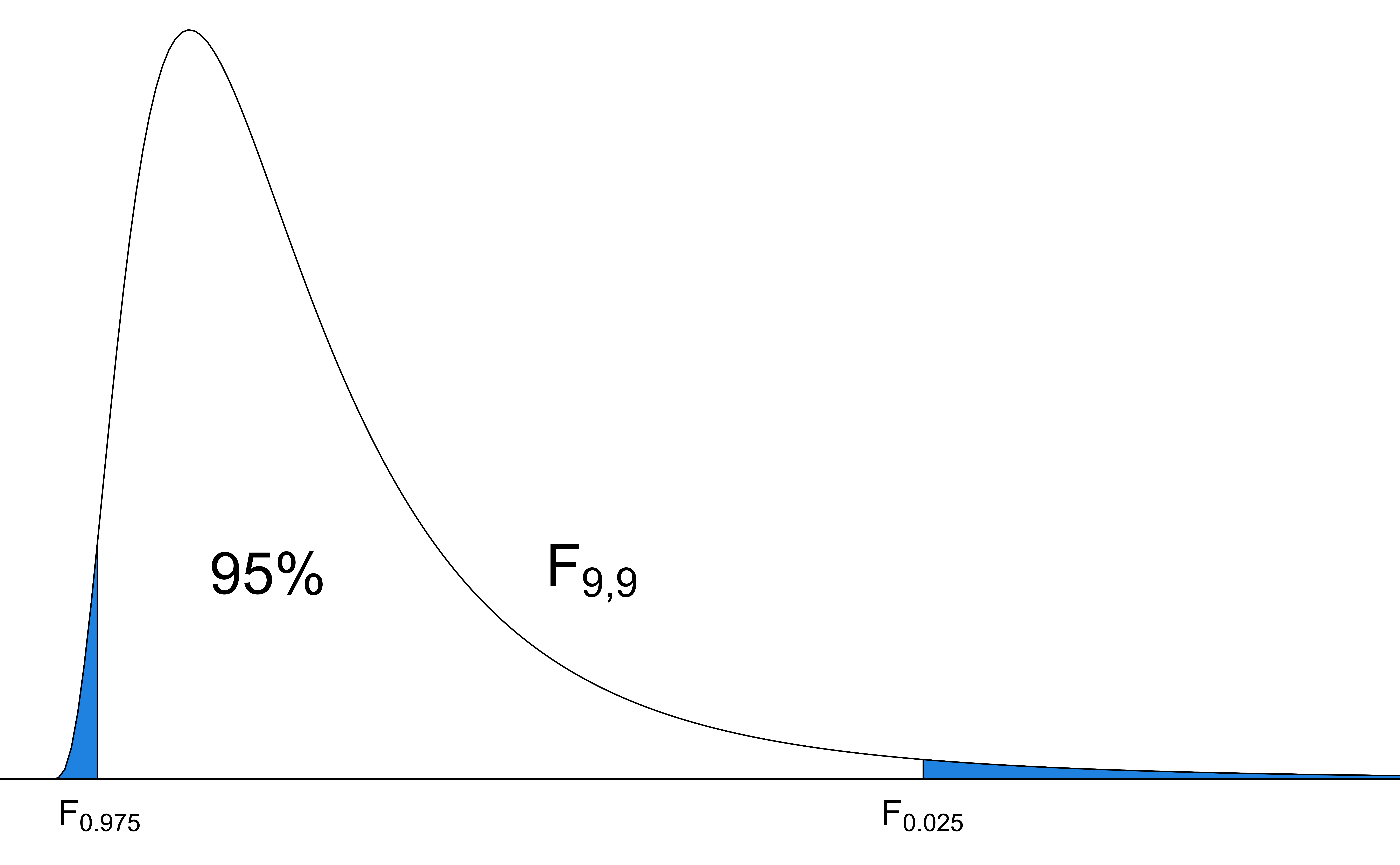
• Step 4-c: Two-tailed test. The critical value is \(F_{0.05/2, \, 10-1, \, 10-1} = 4.03\) or \(F_{1-0.05/2, \, 10-1, \, 10-1} = 0.25\).

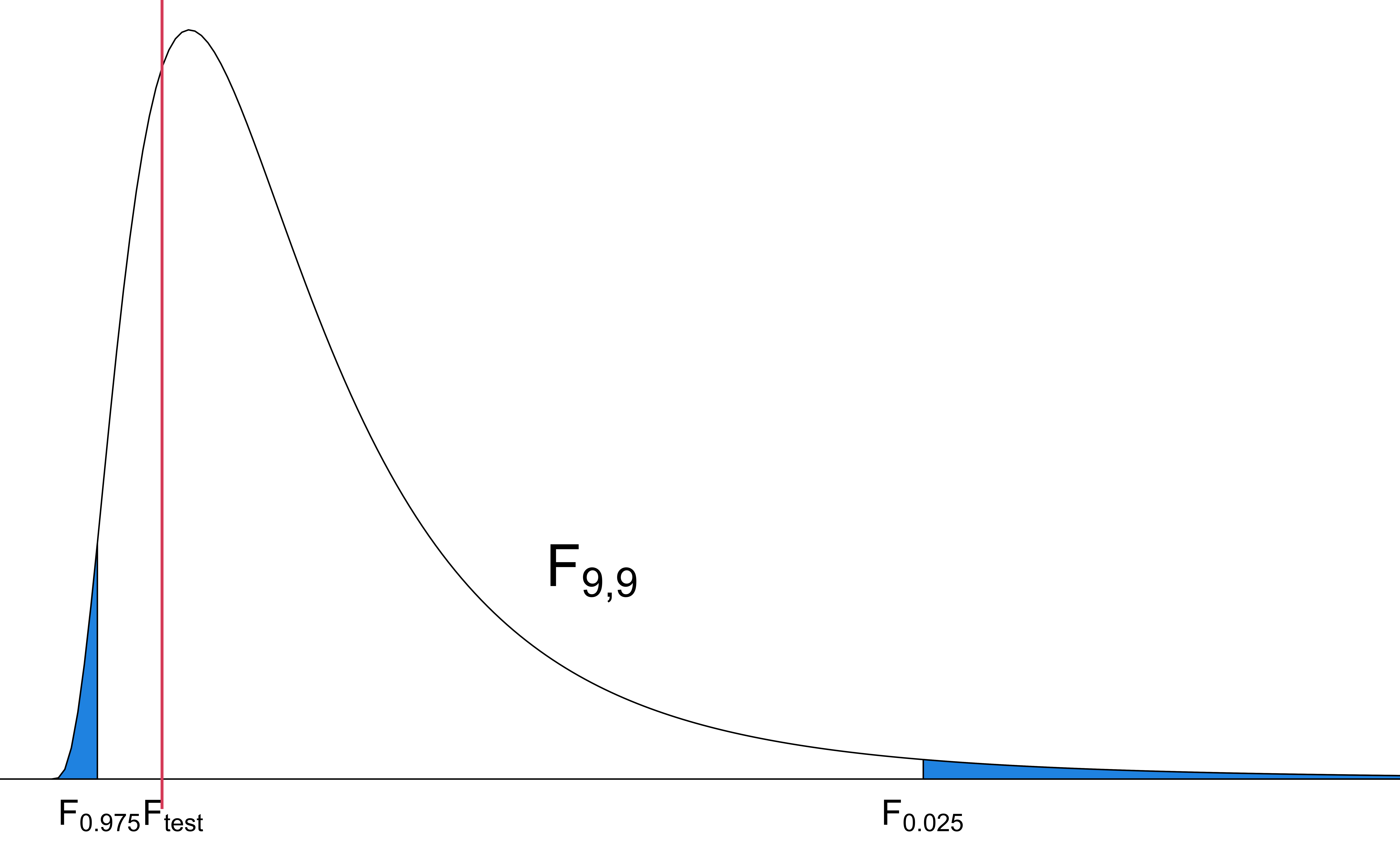
• Step 5-c: Is \(F_{test} > 4.03\) or \(F_{test} < 0.25\)? No.

• Step 6: The evidence is not sufficient to reject the claim that \(\sigma_1 = \sigma_2\).

Back to the Weight Loss Example: 95% CI for \(\sigma_1^2 / \sigma_2^2\)

• The 95% CI for \(\sigma_1^2 / \sigma_2^2\) is \[\small \begin{align} &\left( \frac{s_1^2/s_2^2}{F_{\alpha/2, \, df_1, \, df_2}}, \frac{s_1^2/s_2^2}{F_{1-\alpha/2, \, df_1, \, df_2}} \right) \\ &= \left( \frac{0.51}{4.03}, \frac{0.51}{0.25} \right) = \left(0.13, 2.04\right)\end{align}\]
• We are 95% confident that the ratio \(\sigma_1^2 / \sigma_2^2\) is between 0.13 and 2.04.

Implementing F-test in R

n1 <- 10; n2 <- 10
s1 <- 0.5; s2 <- 0.7
al <- 0.05

## 95% CI for sigma_1^2 / sigma_2^2
f_small <- qf(p = al / 2, 
              df1 = n1 - 1, df2 = n2 - 1, 
              lower.tail = TRUE)
f_big <- qf(p = al / 2, 
            df1 = n1 - 1, df2 = n2 - 1, 
            lower.tail = FALSE)

## lower bound
(s1 ^ 2 / s2 ^ 2) / f_big

[1] 0.127

## upper bound
(s1 ^ 2 / s2 ^ 2) / f_small

[1] 2.05

## Testing sigma_1 = sigma_2
(test_stats <- s1 ^ 2 / s2 ^ 2)

[1] 0.51

(cri_big <- qf(p = al / 2, 
               df1 = n1 - 1, 
               df2 = n2 - 1, 
               lower.tail = FALSE))

[1] 4.03

(cri_small <- qf(p = al / 2, 
                 df1 = n1 - 1, 
                 df2 = n2 - 1, 
                 lower.tail = TRUE))

[1] 0.248

# var.test(x, y, alternative = "two.sided")