Analysis of Variance (ANOVA)

MATH 4720/MSSC 5720 Introduction to Statistics

Dr. Cheng-Han Yu
Department of Mathematical and Statistical Sciences
Marquette University

One-Way Analysis of Variance (ANOVA)

• Rationale

• Procedure

• Examples

ANOVA Rationale

Comparing More Than Two Population Means

In many research settings, we’d like to compare 3 or more population means.

• 4 types of devices used to determine the pH of soil samples.

• Determine whether there are differences in the mean readings of those 4 devices.

• Do different treatments (None, Fertilizer, Irrigation, Fertilizer and Irrigation) affect the mean weights of poplar trees?

• In Chapter 6 we learned methods for comparing 2 population means.

One-Way Analysis of Variance

• A factor is a property or characteristic (categorical variable) that allows us to distinguish the different populations from one another.

• Type of devices and treatment of trees are factors.

• One-way ANOVA examines the effect of a categorical variable on the mean of a numerical variable (response).

• We use analysis of variance to test the equality of 3 or more population means. 🤔

• The method is one-way because we use one single property (categorical variable) for categorizing the populations.

• A treatment (or factor) can be a category or level of a categorical variable.

Requirements of One-Way ANOVA

• The populations of each category are normally distributed.

• The populations have the same variance \(\sigma^2\) (two-sample pooled \(t\)-test).

• The samples are random samples.

• The samples are independent of each other. (not matched or paired in any way)

• The method can still work fairly well when the variances are not equal, unless they are differ by large amounts.

Rationale for ANOVA

Data 1 and Data 2 have the same group sample means \(\bar{y}_1\), \(\bar{y}_2\) and \(\bar{y}_3\) denoted as red dots.

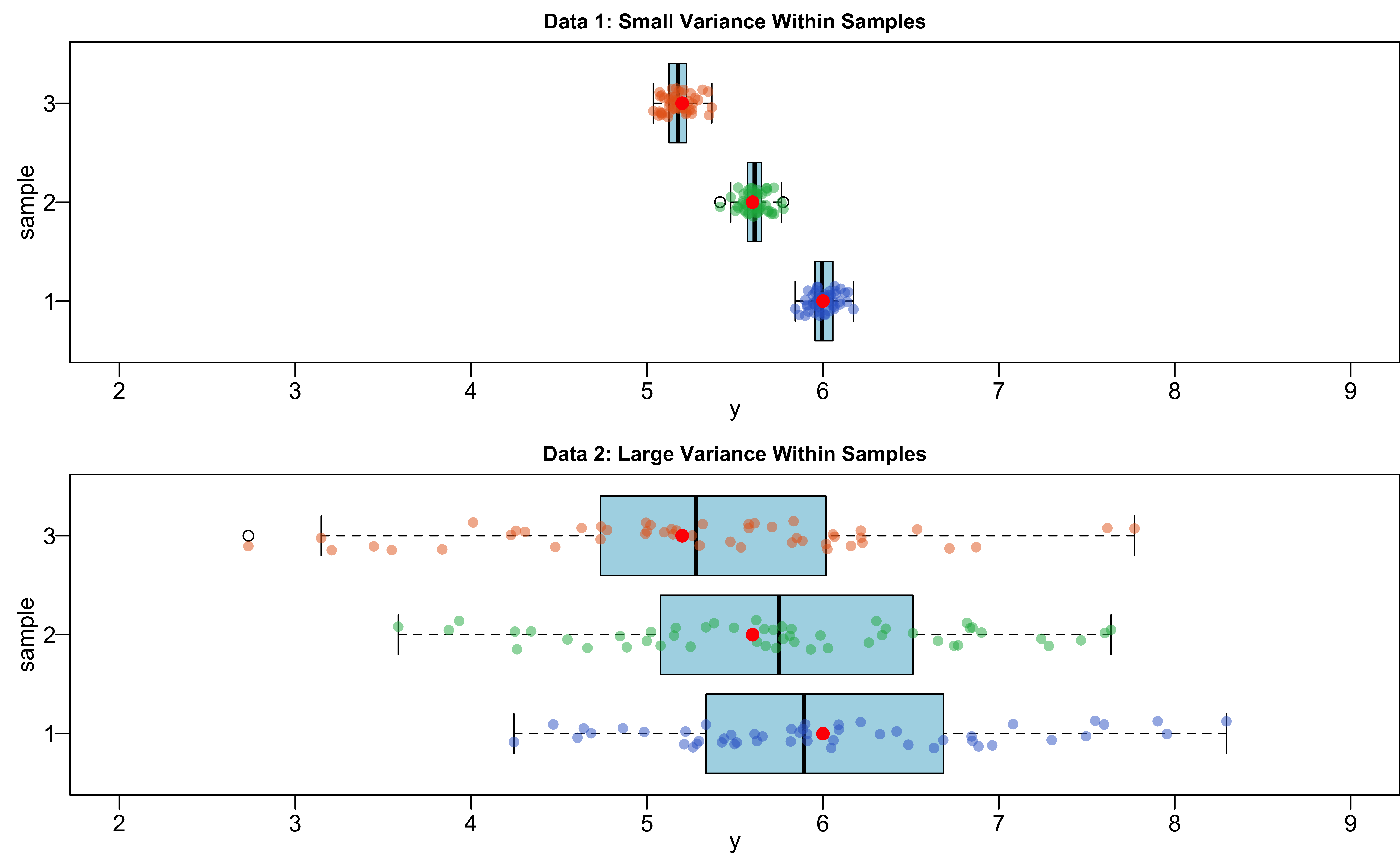
Which data you are more confident to say the population means \(\mu_1\), \(\mu_2\) and \(\mu_3\) are not all the same?

• The boxplots clearly show this difference.
• The 2 data sets have the same group means, but the variance within groups for data 2 is much greater than the variance within groups for data 1.
• The difference in sample means in Data 1 is more likely due to the true difference in population means.
• variation between samples is measured by the pairwise distance among the sample means.
• variation within samples is measured by the how far away the data points away from each other in each sample group.

Variation Between Samples & Variation Within Samples

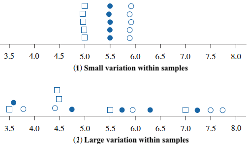
• Data 1: Variability between samples is large in comparison to the variation within samples.

• Data 2: Variation between samples is small relatively to the variation within samples.

More confident to conclude there is a difference in population means when variation between samples is relatively larger than variation within samples.

=> population means are different.

=> less likely and confident to conclude there is a difference in population means.

• When variation within samples relatively larger than the variation between samples, it’s more difficult to distinguish or disentangle one sample from another.

ANOVA Procedures

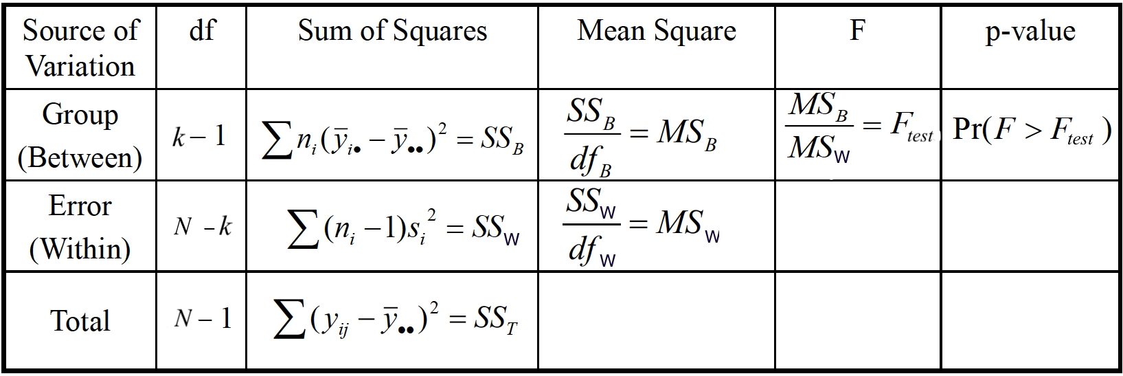
ANOVA Table

ANOVA Data

• There are 5 populations.

• Within each population, 4 data points are collected.

• Data \(y_{ij}\) is the the \(j\)-th data point in the \(i\)-th group.

Population	Data	Sample Mean	Population Mean
1	\(y_{11}\) \(\quad\) \(y_{12}\) \(\quad\) \(y_{13}\) \(\quad\) \(y_{14}\)	\(\bar{y}_{1}\)	\(\mu_{1}\)
2	\(y_{21}\) \(\quad\) \(y_{22}\) \(\quad\) \(y_{23}\) \(\quad\) \(y_{24}\)	\(\bar{y}_{2}\)	\(\mu_{2}\)
3	\(y_{31}\) \(\quad\) \(y_{32}\) \(\quad\) \(y_{33}\) \(\quad\) \(y_{34}\)	\(\bar{y}_{3}\)	\(\mu_{3}\)
4	\(y_{41}\) \(\quad\) \(y_{42}\) \(\quad\) \(y_{43}\) \(\quad\) \(y_{44}\)	\(\bar{y}_{4}\)	\(\mu_{4}\)
5	\(y_{51}\) \(\quad\) \(y_{52}\) \(\quad\) \(y_{53}\) \(\quad\) \(y_{54}\)	\(\bar{y}_{5}\)	\(\mu_{5}\)

This is NOT a tidy data matrix. We may need to save the data in another format before we do ANOVA.

Procedure of ANOVA

• \(\begin{align} &H_0: \mu_1 = \mu_2 = \cdots = \mu_k\\ &H_1: \text{Population means are not all equal} \end{align}\)

• Statistician Ronald Fisher found a way to define a variable that follows the \(F\) distribution:

\[\frac{\text{variance between samples}}{\text{variance within samples}} \sim F_{df_B,\, df_W}\]

• If variance between samples is larger than variance within samples, i.e., \(F_{test}\) is much greater than 1, as Data 1, we reject \(H_0\).

Key: Define variance between samples and variance within samples so that the ratio is \(F\) distributed.

How do we convert the rationale into a formal testing procedure for the test

Variance Within Samples

• Back to two-sample pooled \(t\)-test with equal variance \(\sigma^2\):

\[s_p^2 = \frac{(n_1-1)s_1^2 + (n_2-1)s_2^2}{n_1 + n_2 - 2}\]

What if general \(k\) samples?

• ANOVA assumes the populations have the same variance \(\sigma_1^2 = \sigma_2^2 = \cdots = \sigma_k^2 = \sigma^2\).

\[\boxed{s_W^2 = \frac{(n_1-1)s_1^2 + (n_2-1)s_2^2 + \cdots + (n_k-1)s_k^2}{n_1 + n_2 + \cdots + n_k - k}}\] where \(s_i^2\), \(i = 1, \dots ,k\), is the sample variance of group \(i\).

• \(s_W^2\) represents a combined estimate of the common variance \(\sigma^2\). It measures variability of the observations within the \(k\) populations.

\(s_i^2 = \frac{\sum_{j=1}^{n_i}\left(y_{ij} - \bar{y}_{i\cdot}\right)^2}{n_i-1}\)

Variance Between Samples

\[\boxed{s^2_{B} = \frac{\sum_{i=1}^k n_i (\bar{y}_{i} - \bar{y}_{})^2}{k-1}}\]

• \(\bar{y}_{i}\) is the \(i\)-th sample mean.

• \(\bar{y}_{}\) is the grand sample mean with all data points in all groups combined.

• \(s^2_{B}\) is also an estimate of \(\sigma^2\) and measures variability among sample means for the \(k\) groups.

• If \(H_0\) is true \((\mu_1 = \cdots = \mu_k = \mu)\), any variation in the sample means is due to chance and randomness, and shouldn’t be too large.

  • \(\bar{y}_{1}, \cdots, \bar{y}_{k}\) should be close each other, and they are close to \(\bar{y}_{}\).

\(s_B^2\) and \(s_W^2\) as Sum of Squares/Degrees of Freedom

• Variance is defined as \(\frac{\text{Sum of Squares}}{\text{Degrees of Freedom}}\), which is also called \(\text{Mean Square (MS)}\)

• \(s_B^2 = \frac{\sum_{i=1}^k n_i (\bar{y}_{i} - \bar{y}_{})^2}{k-1} = \frac{\text{Sum of Squares Between Samples (SSB)}}{df_B} = MSB\)

• \(s_W^2 = \frac{\sum_{i=1}^{k} (n_i - 1)s_i^2}{n_1 + n_2 + \cdots + n_k - k} = \frac{\text{Sum of Squares Within Samples (SSW)}}{df_W} = MSW\) \((N = n_1 + \cdots + n_k)\)

Sum of Squares Identity

\[\text{Total Sum of Squares (SST)} = \sum_{j=1}^{n_i}\sum_{i=1}^{k} \left(y_{ij} - \bar{y}_{}\right)^2 = SSB + SSW\]

\[df_{T} = df_{B} + df_{W} \implies N - 1 = (k-1) + (N - k)\]

Sum of Squares Identity

• \(F_{test} = \frac{MSB}{MSW}\)

• Under \(H_0\), \(\frac{S^2_{B}}{S_W^2} \sim F_{k-1, \, N-k}\)

• Reject \(H_0\) if

  • \(F_{test} > F_{\alpha, \, k - 1,\, N-k}\)
  • \(p\)-value \(P(F_{k - 1,\, N-k} > F_{test}) < \alpha\)

ANOVA Examples

Example

• A hypothesis is that a nutrient “Isoflavones” varies among three types of food: (1) cereals and snacks, (2) energy bars, and (3) veggie burgers.

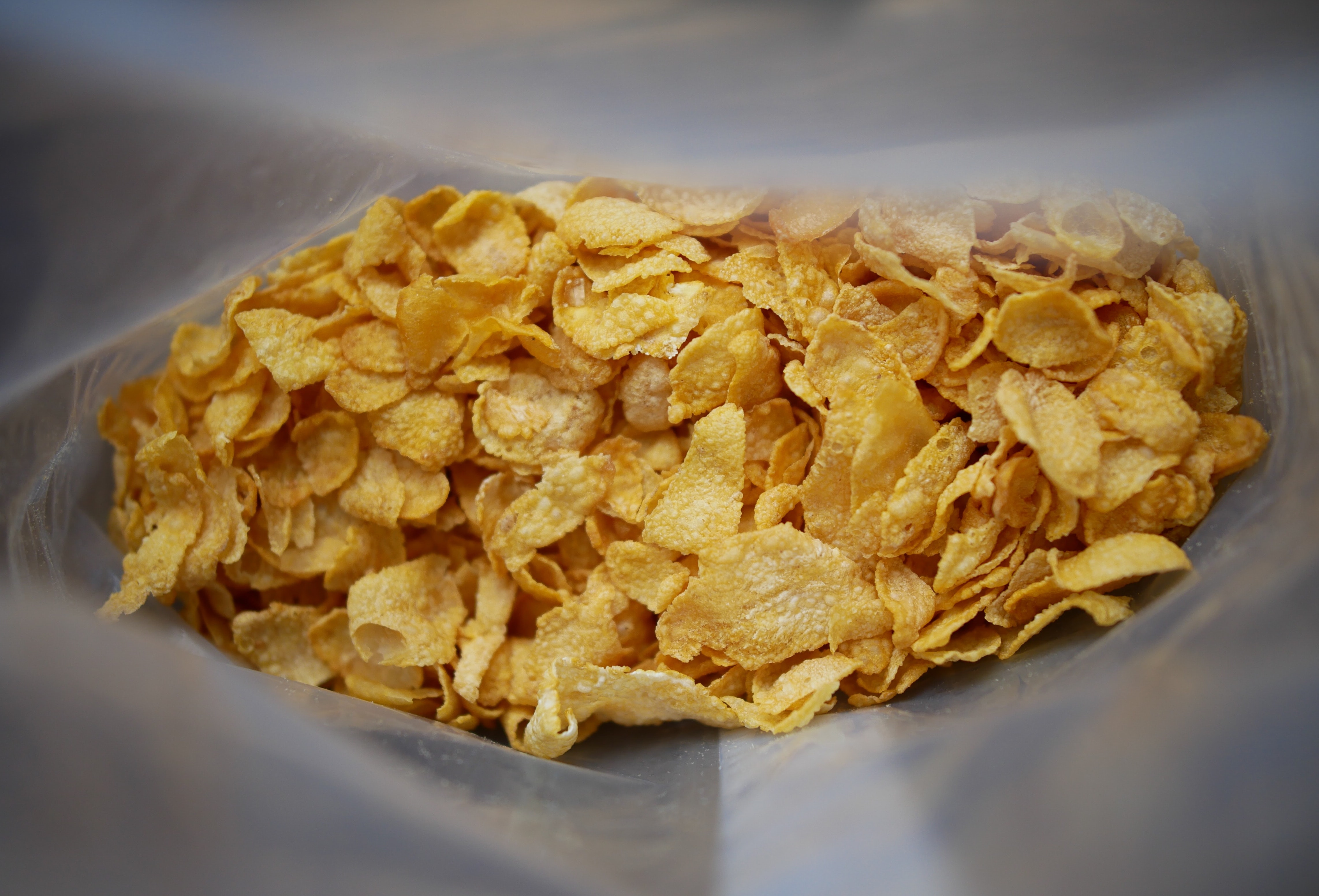
• A sample of 5 each is taken and the amount of isoflavones is measured.

• Is there a sufficient evidence to conclude that the mean isoflavone levels vary among these food items? \(\alpha = 0.05\).

Ask for \(H_0\)

Example - Data

data

   1  2  3
1  3 19 25
2 17 10 15
3 12  9 12
4 10  7  9
5  4  5  8

Here columns represent food items and rows are samples.

So tell me what is the value of \(y_{23}\)!

We prefer data format like

data_anova

    y    food
1   3 cereals
2  17 cereals
3  12 cereals
4  10 cereals
5   4 cereals
6  19  energy
7  10  energy
8   9  energy
9   7  energy
10  5  energy
11 25  veggie
12 15  veggie
13 12  veggie
14  9  veggie
15  8  veggie

── Attaching core tidyverse packages ──────────────────────── tidyverse 2.0.0 ──
✔ dplyr     1.1.4     ✔ readr     2.1.5
✔ forcats   1.0.0     ✔ stringr   1.5.1
✔ ggplot2   4.0.0     ✔ tibble    3.3.0
✔ lubridate 1.9.4     ✔ tidyr     1.3.1
✔ purrr     1.1.0     
── Conflicts ────────────────────────────────────────── tidyverse_conflicts() ──
✖ dplyr::filter() masks stats::filter()
✖ dplyr::lag()    masks stats::lag()
ℹ Use the conflicted package (<http://conflicted.r-lib.org/>) to force all conflicts to become errors

# A tibble: 15 × 2
   food        y
   <chr>   <dbl>
 1 cereals     3
 2 cereals    17
 3 cereals    12
 4 cereals    10
 5 cereals     4
 6 energy     19
 7 energy     10
 8 energy      9
 9 energy      7
10 energy      5
11 veggie     25
12 veggie     15
13 veggie     12
14 veggie      9
15 veggie      8

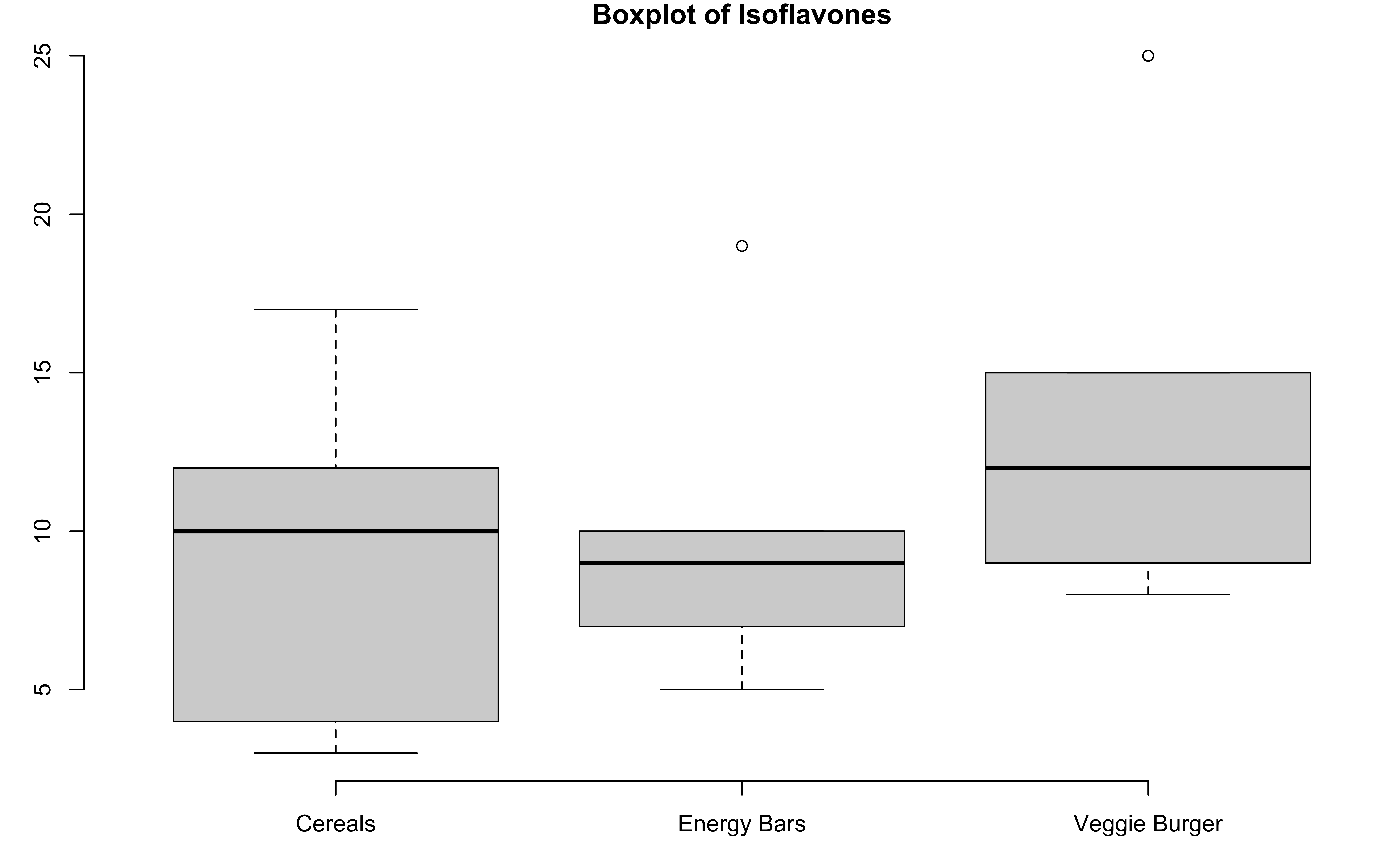
Example - Boxplot

Example - Test Assumptions

• Assumptions:
  • \(\sigma_1 = \sigma_2 = \sigma_3\) (I tested it)
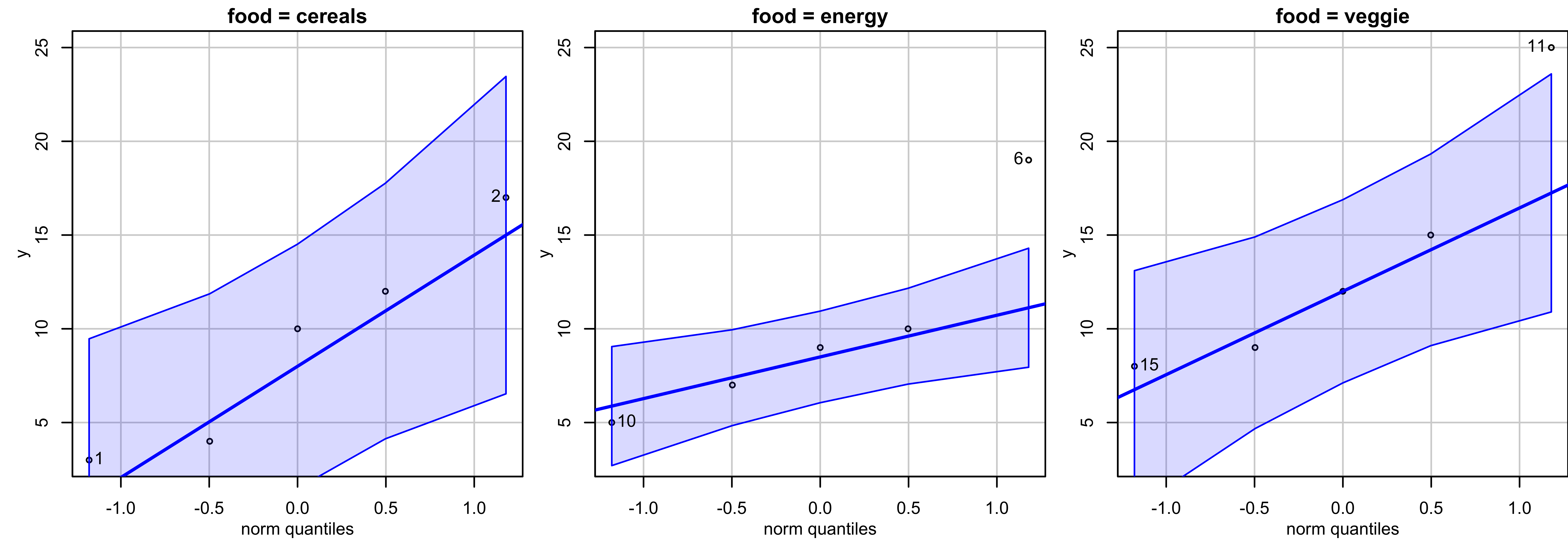
  • Data are generated from a normal distribution for each type of food.

Example - ANOVA Testing

• \(\begin{align}&H_0: \mu_1 = \mu_2 = \mu_3\\&H_1: \mu_is \text{ not all equal} \end{align}\)

😎 Do all calculations and generate an ANOVA table using just one line of code! 🤟 ✌️

Example - ANOVA Table

anova(lm(y ~ food, data = data_anova))

Analysis of Variance Table

Response: y
          Df Sum Sq Mean Sq F value Pr(>F)
food       2   60.4   30.20   0.828   0.46
Residuals 12  437.6   36.47               

    One-way analysis of means

data:  y and food
F = 0.8282, num df = 2, denom df = 12, p-value = 0.46