Please submit your work in onePDF file to D2L > Assessments > Dropbox. Multiple files or a file that is not in pdf format is not allowed.
With your submission, you commit to academic integrity through the following honor pledge:
I recognize the importance of personal integrity in all aspects of life and work. I commit myself to truthfulness, honor and responsibility, by which I earn the respect of others. I support the development of good character and commit myself to uphold the highest standards of academic integrity as an important aspect of personal integrity. My commitment obliges me to conduct myself according to the Marquette University Honor Code.
This exam is to be entirely your own efforts. You may use any resources, including Generative AI tools, while working on this exam. However, you are NOT allowed to discuss the exam with anyone except Dr. Yu, nor may you post any of the exam questions on any platform to solicit answers. Any violation of this policy will be treated as academic misconduct. If you are caught cheating, your case will be reported immediately to the Academic Integrity Council.
In your exam, please number problems/questions in order.
Even if you use R to compute your final answer, you must show your calculation steps and/or explain your reasoning in order to receive full credit.
Handwritten tables and figures receive no credits.
Exam Problems (50 points)
[30 points] A Marquette professor of College of Education believes that Marquette engineering students are talented and their mean ACT score is greater than 30. She would like to collect evidence of her claim and do a hypothesis testing. Marquette data center director said that the population of ACT score of engineering majors follows a normal distribution with the population variance of value 9.
Is the claim a \(H_0\) or \(H_1\) claim? Write down \(H_0\) and \(H_1\) based on her claim. Is this a left-tailed, right-tailed, or two-tailed test? Please explain.
Due to COVID-19, Marquette’s research budget is cut. The professor’s assistant can only collect a small random sample of size 16. Are one-sample \(z\)-test and/or \(t\)-test procedures appropriate with such a small size? If yes, why? If not, add conditions to make the procedures appropriate.
The assistant never takes MATH 4720 and she only remembers that the professor said 31.7 is the threshold value to be compared with the observed sample mean \(\overline{x}\). Should she reject \(H_0\) when \(\bar{x} > 31.7\) or when \(\bar{x} < 31.7\)? Please explain.
Given the rejection region in (c), write down the definition of the Type I error rate in the problem and determine its value.
If the \(p\)-value is 0.1, what is the value of observed sample mean \(\overline{x}\)?
Based on (c), (d), (e), Is \(H_0\) rejected?
# ------------## (a) # ------------# right-tailed, H1 claim# H0: mu <= 30# H1: mu > 30# ------------## (b) # ------------# yes because the ACT score is normally distributed# ------------## (c) # ------------# x_bar > 31.7 because it is a right-tailed test# ------------## (d)# ------------# type I error rate = P(reject H0 | H0 is true)mu0<-30; x_bar_cv<-31.7; sig2<-9; n<-16pnorm((x_bar_cv-mu0)/sqrt(sig2/n), lower.tail =FALSE)
[1] 0.0117053
# ------------## (e)# ------------p_val<-0.1qnorm(p_val, mean =mu0, sd =sqrt(sig2/n), lower.tail =FALSE)
[1] 30.96116
# ------------## (f)# ------------# Do not reject H0# There is insufficient evidence to support the claim that engineering students has mean ACT > 30.# ------------## (g) # ------------# type II error rate = P(do not reject H0 | H0 is false)x_bar_cv_new<-31.5mu1<-31pnorm((x_bar_cv_new-mu1)/sqrt(sig2/n))
[1] 0.7475075
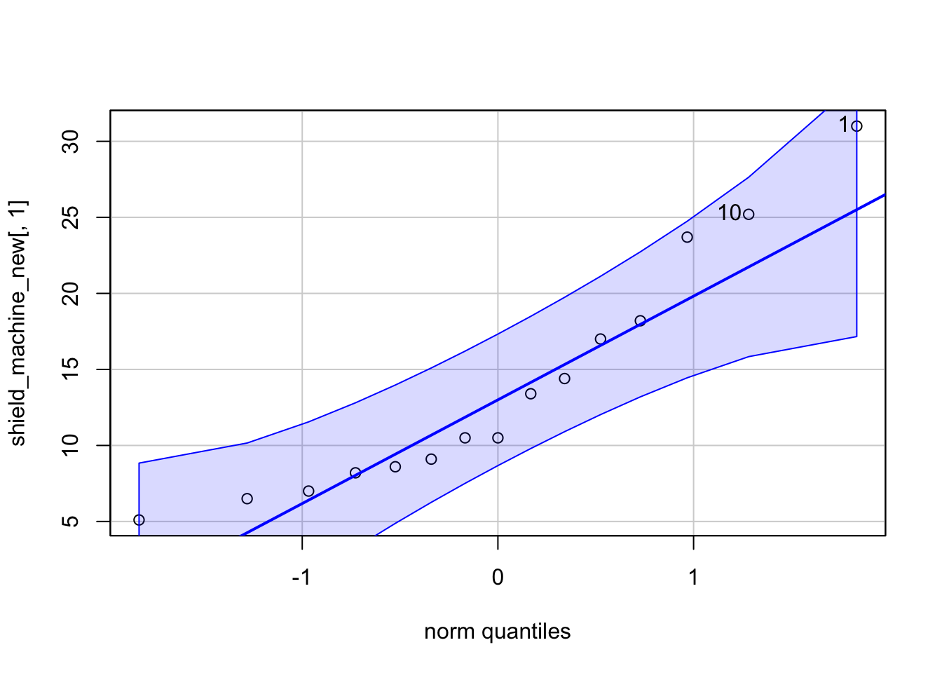
[20 points] A corporation in Chicago makes insulation shields for electrical wires using three types of machines. The company wants to evaluate the variation in the inside diameter dimensions of the shields produced by the machine A, B and C. A quality control engineer randomly selects shields produced by each of the machines and records the inside diameter of each shield (in millimeters), as shown in Table 1. The data can be downloaded at shield_machine.csv. She wants to determine whether the mean diameter produced by the three machines differ.
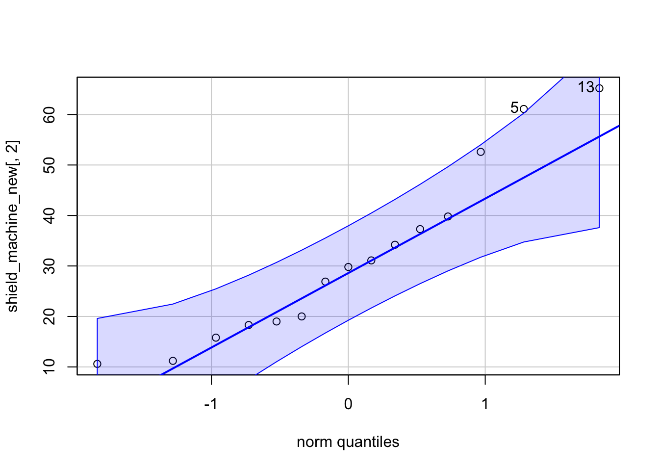
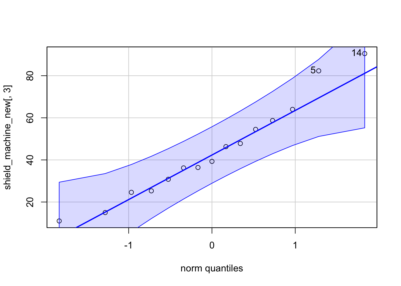
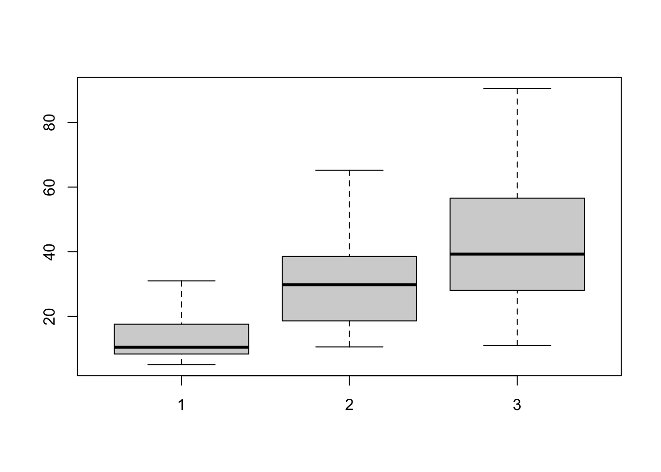
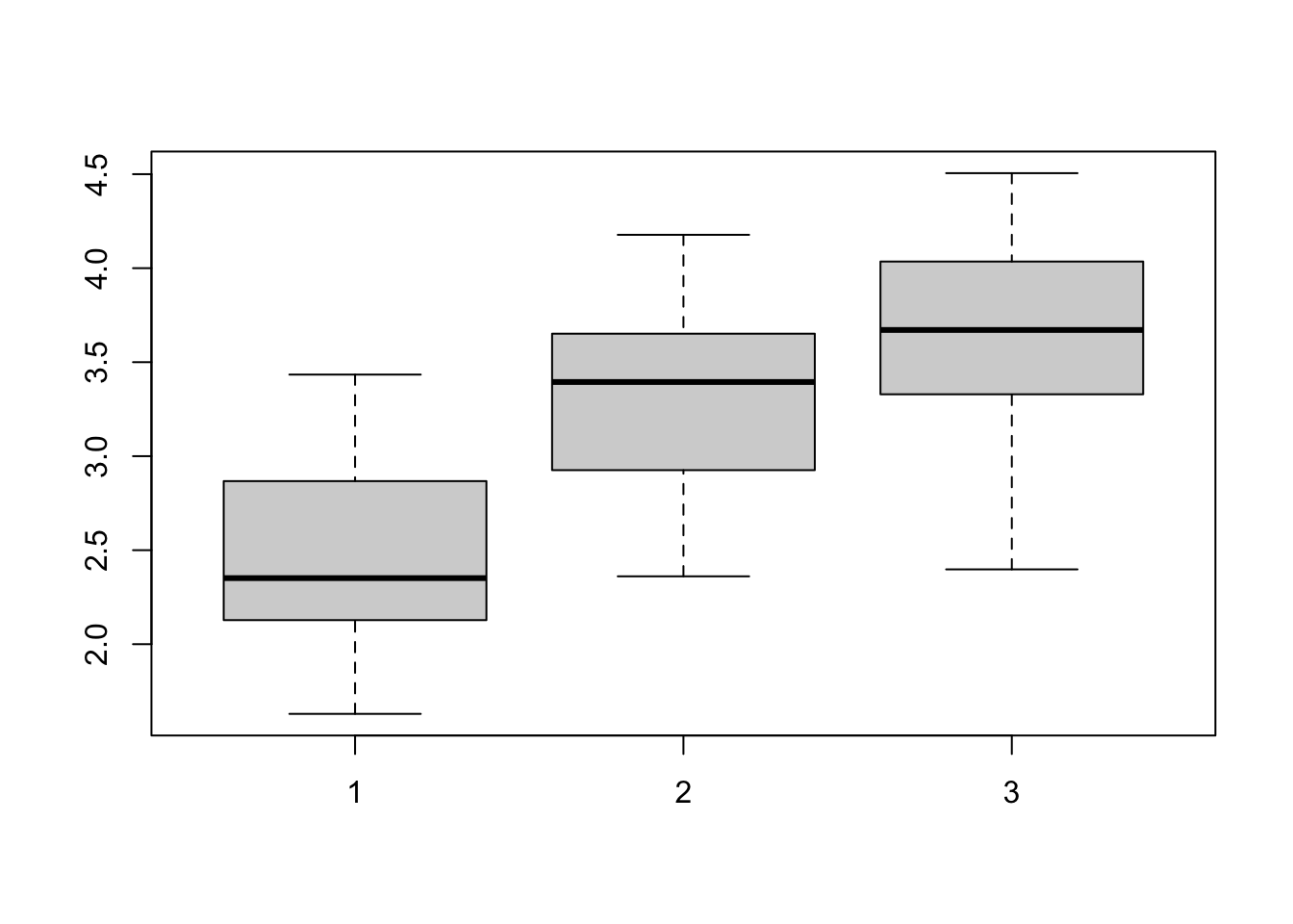
Check normality and homogeneity of variance using QQ-plot and boxplot. Comment on your plots.
Based on your findings in (a), would it be appropriate to proceed with an analysis of variance (ANOVA)? Please explain.
If your answer is YES in (b), conduct ANOVA on the original data. If NOT, do the natural log (log with base \(e = 2.71828...\)) transformation on the data and show the transformed data satisfy ANOVA assumptions. Then conduct ANOVA on the transformed data. Show the ANOVA table and determine whether the mean diameters differ.
Table 1: Sampled data of the inside diameter of shields produced by machine A, B and C.
# not very normal but OKboxplot(shield_machine_new)
## variances are not homogeneous# ------------## (b)# ------------## Not appropriate because ANONA requires normality of data and homogeneous variances.# ------------## (d)# ------------apply(shield_machine_new, 2, var)
# fitted_val_log <- matrix(lm_res_log$fitted.values, 15, 3)# colnames(fitted_val_log) <- c("A", "B", "C")# qqPlot(lm_res_log$residuals, pch = 19, id = FALSE, ylab = "residuals", # main = "Normal Probability Plot for Residuals")# plot(lm_res_log$fitted.values, lm_res_log$residuals, xlab = "Fitted Value",# ylab = "Residual", main = "Versus Fits", pch = 19, col = "red")# abline(h = 0)## another way# aov_res <- aov(diameter ~ machine, data = data_sim_log)# summary(aov_res)
AI Usage Declaration. Using GenAI is permitted for this course. If you choose to use GenAI to assist with your exam, you must include a brief statement documenting your use. Please provide the following information:
Why/How I Used AI Why do you need to use GenAI? Which tool did you use? Describe your prompts or questions. What and how did you ask the AI to help you?
Generated Output Include a screenshot or excerpt (copy and paste) of the AI’s response.
How I Used the Output Did you revise it? Did you use it directly, or compare it with your answers? What decisions did you make based on the output?